Chi-squared test: Independence and Goodness of Fit
Chester Ismay and Andrew Bray
2019-11-19
Source:vignettes/chisq_test.Rmd
chisq_test.RmdNote: The type argument in generate() is automatically filled based on the entries for specify() and hypothesize(). It can be removed throughout the examples that follow. It is left in to reiterate the type of generation process being performed.
Data preparation
library(nycflights13)
library(dplyr)
library(ggplot2)
library(stringr)
library(infer)
set.seed(2017)
fli_small <- flights %>%
  na.omit() %>%
  sample_n(size = 500) %>%
  mutate(season = case_when(
    month %in% c(10:12, 1:3) ~ "winter",
    month %in% c(4:9) ~ "summer"
  )) %>%
  mutate(day_hour = case_when(
    between(hour, 1, 12) ~ "morning",
    between(hour, 13, 24) ~ "not morning"
  )) %>%
  select(arr_delay, dep_delay, season,
day_hour, origin, carrier)- Two numeric -
arr_delay,dep_delay - Two categories
-
season("winter","summer"), -
day_hour("morning","not morning")
-
- Three categories -
origin("EWR","JFK","LGA") - Sixteen categories -
carrier
A test of independence
Say we wish to assess whether flights out of the three NYC airports have a seasonal component; whether La Guardia gets relatively more winter traffic, say, than JFK. This could be formulated as a test of independence between the origin (airport) and season variables.
Calculate observed statistic
The recommended approach is to use specify() %>% calculate():
obs_chisq <- fli_small %>%
  specify(origin ~ season) %>% # alt: response = origin, explanatory = season
  calculate(stat = "Chisq")
The observed \(\chi^2\) statistic is 1.7926106.
There also exists a shortcut:
Sampling distribution under null (via simulation)
Under the null hypothesis that origin is independent of season, we can simulate the distribution of \(\chi^2\) statistics.
chisq_null_perm <- fli_small %>%
  specify(origin ~ season) %>% # alt: response = origin, explanatory = season
  hypothesize(null = "independence") %>%
  generate(reps = 1000, type = "permute") %>%
  calculate(stat = "Chisq")

visualize(chisq_null_perm) +
  shade_p_value(obs_stat = obs_chisq, direction = "greater")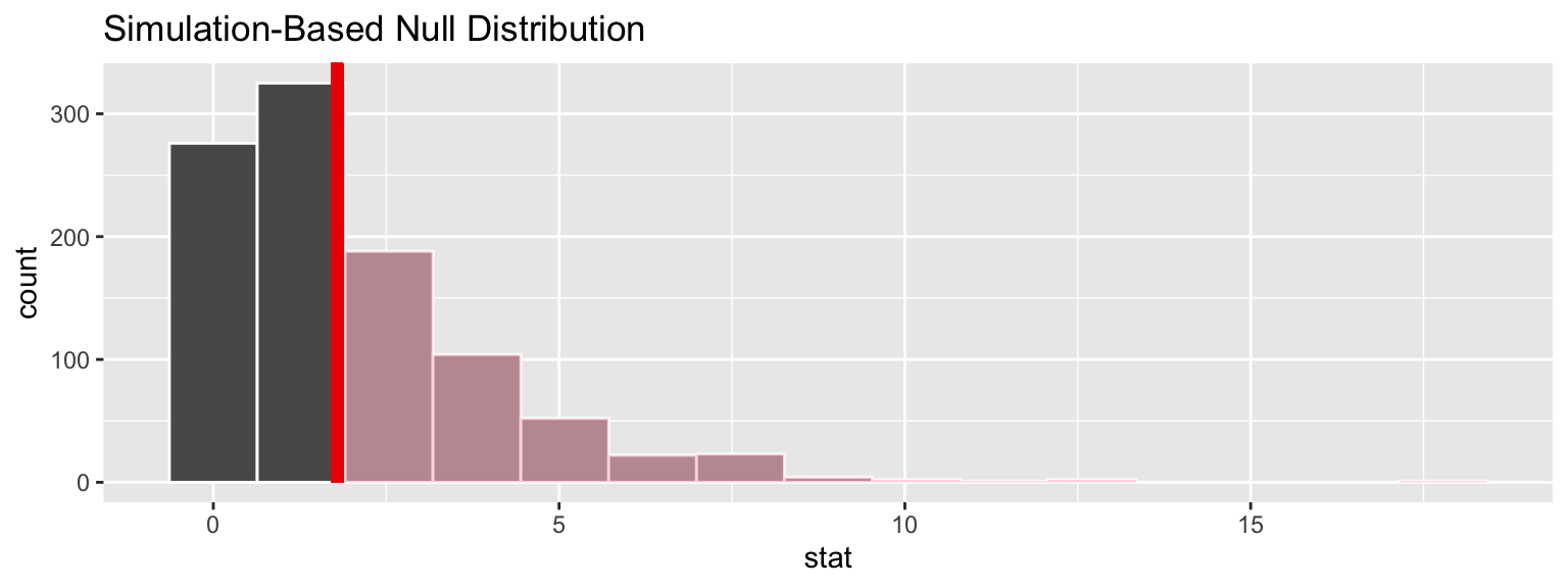
Sampling distribution under null (via approximation)
chisq_null_theor <- fli_small %>%
  specify(origin ~ season) %>%
  hypothesize(null = "independence") %>%
  # generate() ## Not used for theoretical
  calculate(stat = "Chisq")

visualize(chisq_null_theor, method = "theoretical") +
  shade_p_value(obs_stat = obs_chisq, direction = "right")
## Warning: Check to make sure the conditions have been met for the
## theoretical method. {infer} currently does not check these for you.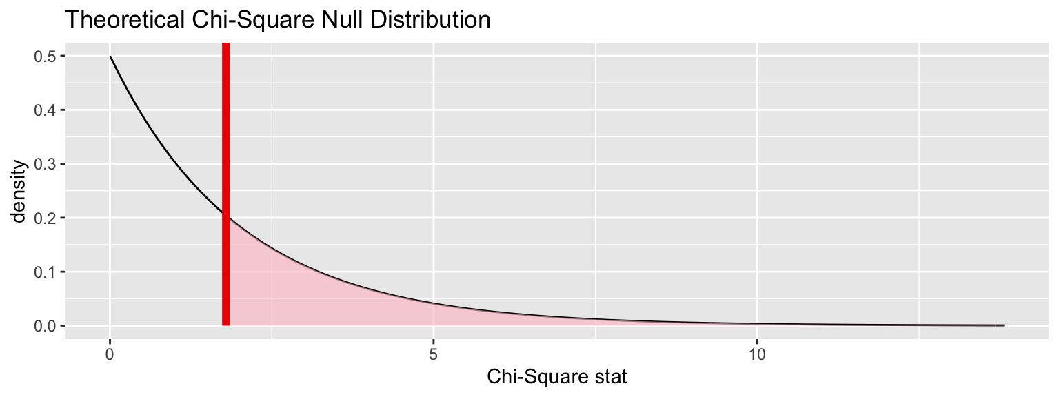
We can also overlay the appropriate \(\chi^2\) distribution on top of permuted statistics.
visualize(chisq_null_perm, method = "both") +
  shade_p_value(obs_stat = obs_chisq, direction = "right")
## Warning: Check to make sure the conditions have been met for the
## theoretical method. {infer} currently does not check these for you.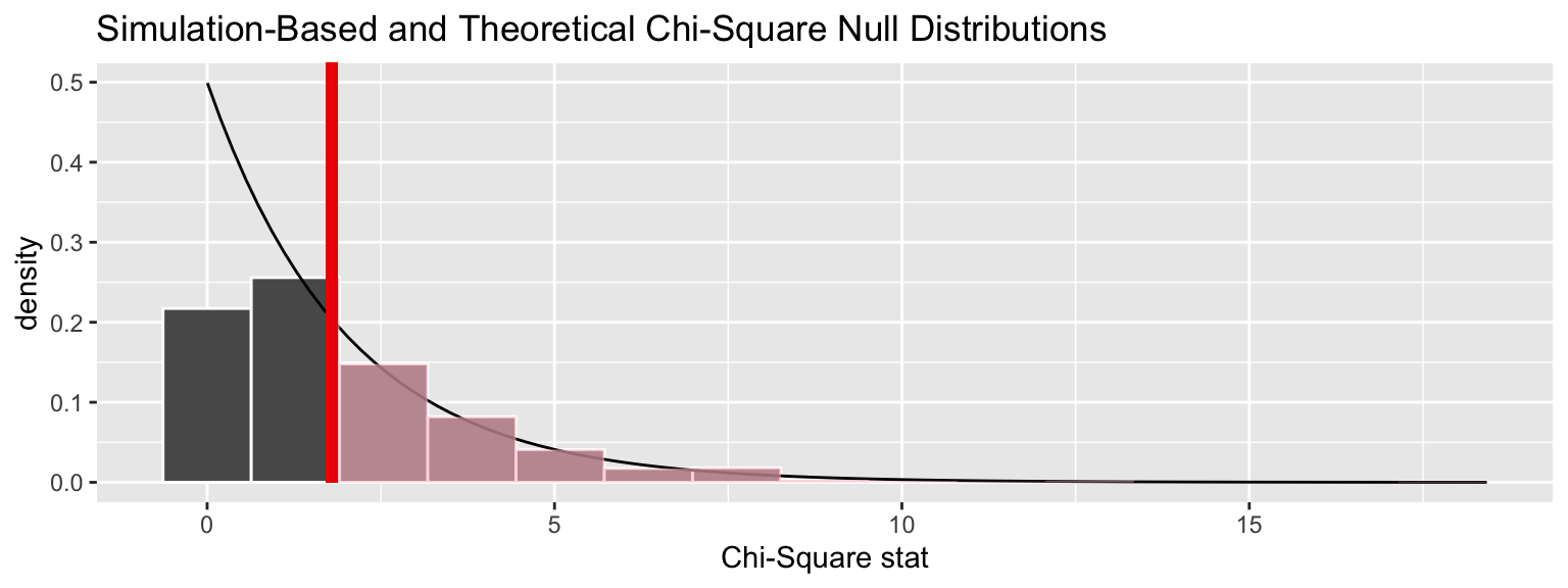
Goodness of fit test
The \(\chi^2\) is also useful for determining how different the observed distribution of a single categorical variable is from a proposed theoretical distribution. Let’s test the (trivial) null hypothesis that there is no variability in number of flights that leave from the three NYC area airports. Said another way, we hypothesize that a flat distribution over the airports is a good fit for our data.
Sampling distribution under null (via simulation)
chisq_null_perm <- fli_small %>%
  specify(response = origin) %>%
  hypothesize(null = "point",
              p = c("EWR" = .33, "JFK" = .33, "LGA" = .34)) %>%
  generate(reps = 1000, type = "simulate") %>%
  calculate(stat = "Chisq")

visualize(chisq_null_perm) +
  shade_p_value(obs_stat = obs_chisq, direction = "greater")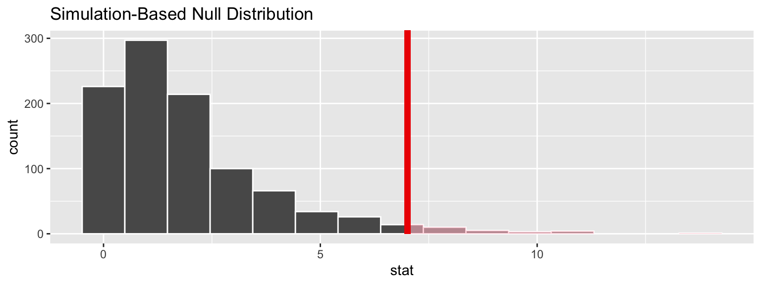
Sampling distribution under null (via approximation)
chisq_null_theor <- fli_small %>%
  specify(response = origin) %>%
  hypothesize(null = "point",
              p = c("EWR" = .33, "JFK" = .33, "LGA" = .34)) %>%
  calculate(stat = "Chisq")

visualize(chisq_null_theor, method = "theoretical") +
  shade_p_value(obs_stat = obs_chisq, direction = "right")
## Warning: Check to make sure the conditions have been met for the
## theoretical method. {infer} currently does not check these for you.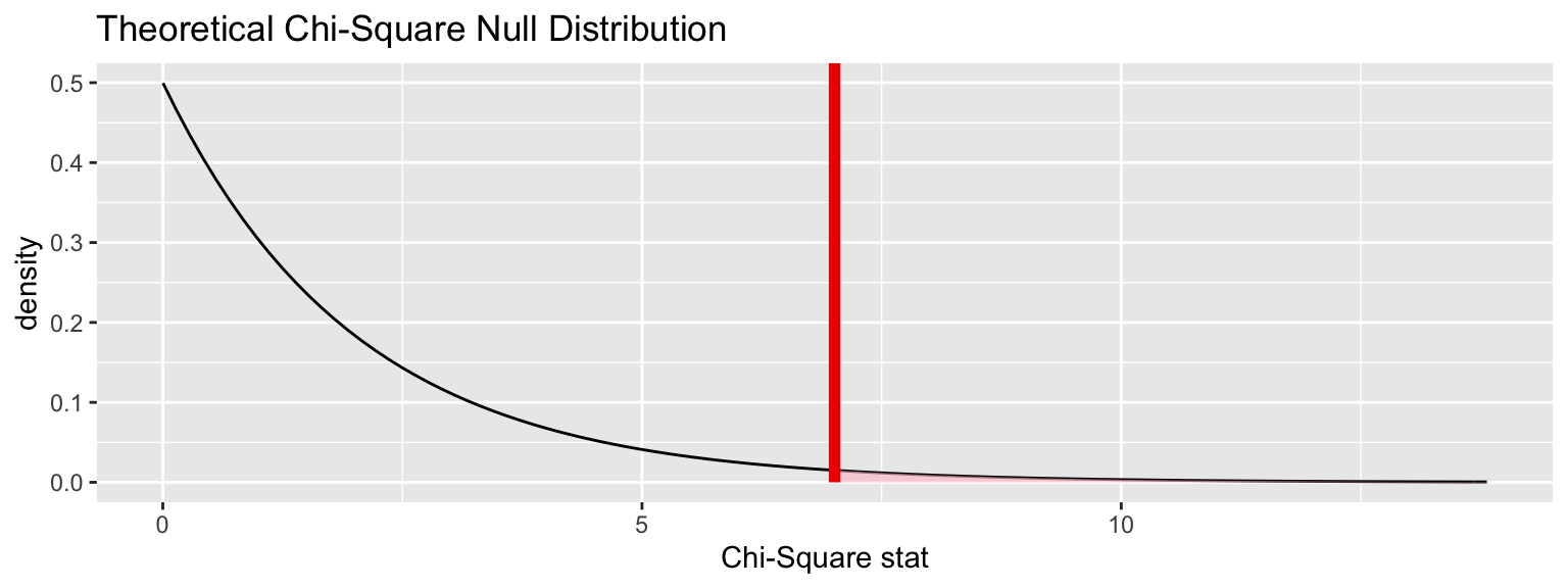
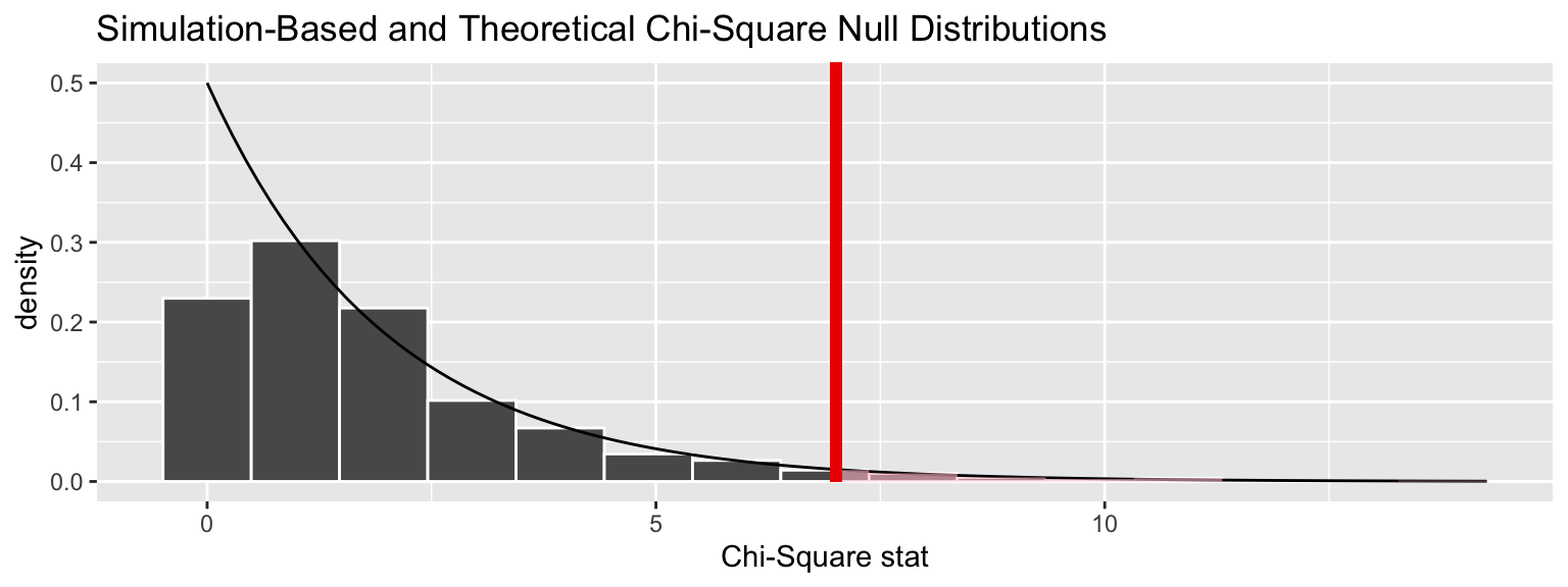
We can also overlay the appropriate \(\chi^2\) distribution on top of permuted statistics.
visualize(chisq_null_perm, method = "both") +
  shade_p_value(obs_stat = obs_chisq, direction = "right")
## Warning: Check to make sure the conditions have been met for the
## theoretical method. {infer} currently does not check these for you.