Full infer pipeline examples using nycflights13 flights data
Chester Ismay
Updated on 2018-06-14
Source:vignettes/observed_stat_examples.Rmd
observed_stat_examples.RmdData preparation
library(nycflights13)
library(dplyr)
library(ggplot2)
library(stringr)
library(infer)
set.seed(2017)
fli_small <- flights %>%
  na.omit() %>%
  sample_n(size = 500) %>%
  mutate(season = case_when(
    month %in% c(10:12, 1:3) ~ "winter",
    month %in% c(4:9) ~ "summer"
  )) %>%
  mutate(day_hour = case_when(
    between(hour, 1, 12) ~ "morning",
    between(hour, 13, 24) ~ "not morning"
  )) %>%
  select(arr_delay, dep_delay, season,
day_hour, origin, carrier)- Two numeric -
arr_delay,dep_delay - Two categories
-
season("winter","summer"), -
day_hour("morning","not morning")
-
- Three categories -
origin("EWR","JFK","LGA") - Sixteen categories -
carrier
Hypothesis tests
One numerical variable (mean)
Observed stat
## # A tibble: 1 x 1
##    stat
##   <dbl>
## 1  11.5
null_distn <- fli_small %>%
specify(response = dep_delay) %>%
hypothesize(null = "point", mu = 10) %>%
generate(reps = 1000) %>%
calculate(stat = "mean")## Setting `type = "bootstrap"` in `generate()`.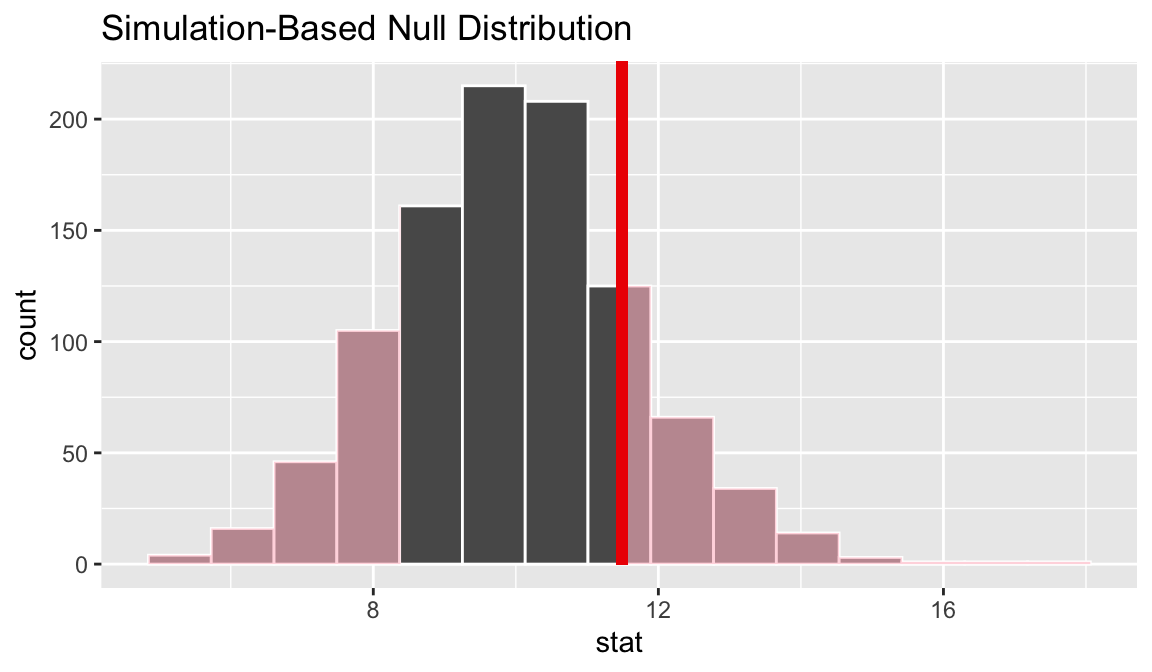
## # A tibble: 1 x 1
##   p_value
##     <dbl>
## 1   0.356
One numerical variable (standardized mean \(t\))
Observed stat
null_distn <- fli_small %>%
  specify(response = dep_delay) %>%
  hypothesize(null = "point", mu = 8) %>%
  generate(reps = 1000) %>%
  calculate(stat = "t")
## Setting `type = "bootstrap"` in `generate()`.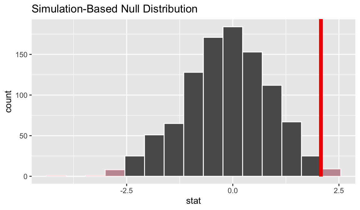
## # A tibble: 1 x 1
##   p_value
##     <dbl>
## 1   0.018
One numerical variable (median)
Observed stat
## # A tibble: 1 x 1
##    stat
##   <dbl>
## 1    -2
null_distn <- fli_small %>%
specify(response = dep_delay) %>%
hypothesize(null = "point", med = -1) %>%
generate(reps = 1000) %>%
calculate(stat = "median")## Setting `type = "bootstrap"` in `generate()`.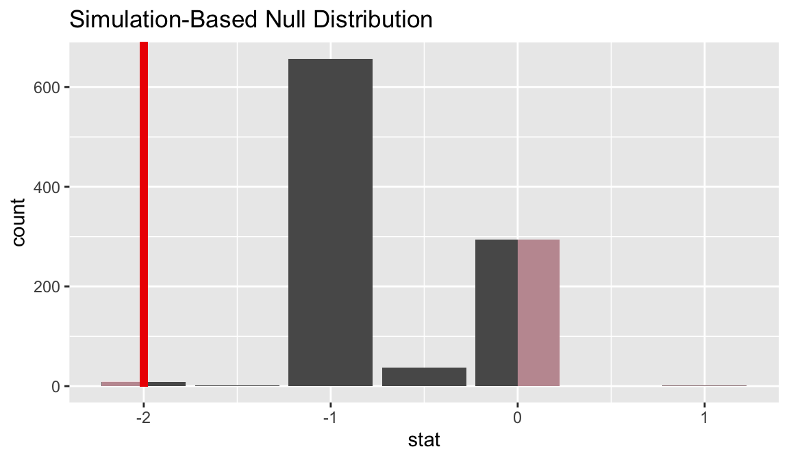
## # A tibble: 1 x 1
##   p_value
##     <dbl>
## 1   0.018
One categorical (one proportion)
Observed stat
( p_hat <- fli_small %>%
  specify(response = day_hour, success = "morning") %>%
  calculate(stat = "prop") )
## # A tibble: 1 x 1
## stat
## <dbl>
## 1 0.452null_distn <- fli_small %>%
specify(response = day_hour, success = "morning") %>%
hypothesize(null = "point", p = .5) %>%
generate(reps = 1000) %>%
calculate(stat = "prop")## Setting `type = "simulate"` in `generate()`.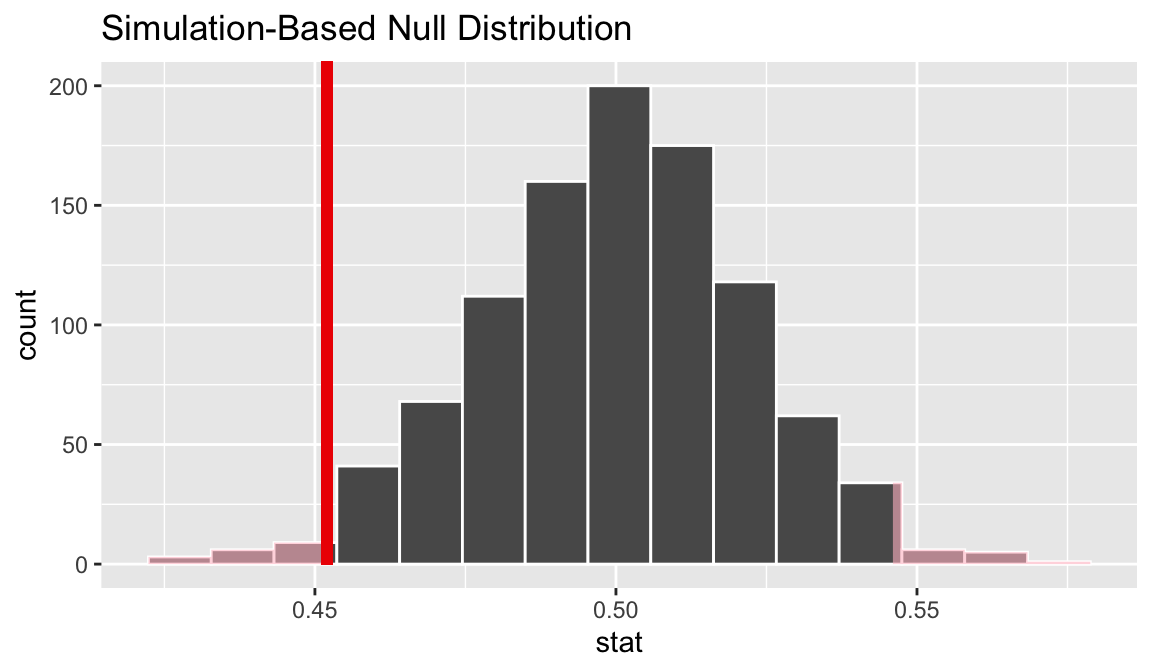
## # A tibble: 1 x 1
##   p_value
##     <dbl>
## 1   0.036
Logical variables will be coerced to factors:
null_distn <- fli_small %>%
  mutate(day_hour_logical = (day_hour == "morning")) %>%
  specify(response = day_hour_logical, success = "TRUE") %>%
  hypothesize(null = "point", p = .5) %>%
  generate(reps = 1000) %>%
  calculate(stat = "prop")
## Setting `type = "simulate"` in `generate()`.Two categorical (2 level) variables
Observed stat
( d_hat <- fli_small %>%
  specify(day_hour ~ season, success = "morning") %>%
  calculate(stat = "diff in props", order = c("winter", "summer")) )
## # A tibble: 1 x 1
## stat
## <dbl>
## 1 0.00438null_distn <- fli_small %>%
specify(day_hour ~ season, success = "morning") %>%
hypothesize(null = "independence") %>%
generate(reps = 1000) %>%
calculate(stat = "diff in props", order = c("winter", "summer"))## Setting `type = "permute"` in `generate()`.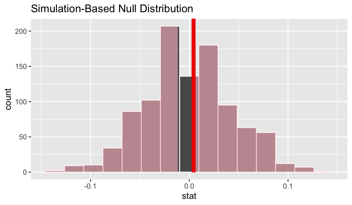
## # A tibble: 1 x 1
## p_value
## <dbl>
## 1 0.954Two categorical (2 level) variables (z)
Standardized observed stat
( z_hat <- fli_small %>%
specify(day_hour ~ season, success = "morning") %>%
calculate(stat = "z", order = c("winter", "summer")) )## # A tibble: 1 x 1
## stat
## <dbl>
## 1 0.0985null_distn <- fli_small %>%
specify(day_hour ~ season, success = "morning") %>%
hypothesize(null = "independence") %>%
generate(reps = 1000) %>%
calculate(stat = "z", order = c("winter", "summer"))## Setting `type = "permute"` in `generate()`.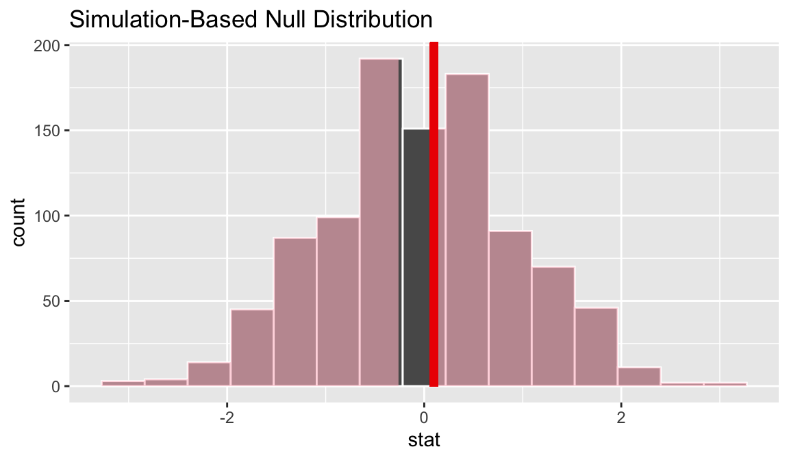
## # A tibble: 1 x 1
## p_value
## <dbl>
## 1 0.95Note the similarities in this plot and the previous one.
One categorical (>2 level) - GoF
Observed stat
Note the need to add in the hypothesized values here to compute the observed statistic.
( Chisq_hat <- fli_small %>%
specify(response = origin) %>%
hypothesize(null = "point",
p = c("EWR" = .33, "JFK" = .33, "LGA" = .34)) %>%
calculate(stat = "Chisq") )## # A tibble: 1 x 1
## stat
## <dbl>
## 1 7.01null_distn <- fli_small %>%
specify(response = origin) %>%
hypothesize(null = "point",
p = c("EWR" = .33, "JFK" = .33, "LGA" = .34)) %>%
generate(reps = 1000, type = "simulate") %>%
calculate(stat = "Chisq")
visualize(null_distn) +
shade_p_value(obs_stat = Chisq_hat, direction = "greater")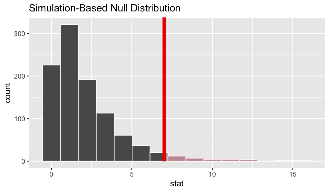
## # A tibble: 1 x 1
## p_value
## <dbl>
## 1 0.037Two categorical (>2 level) variables
Observed stat
## # A tibble: 1 x 1
## stat
## <dbl>
## 1 0.528null_distn <- fli_small %>%
specify(day_hour ~ origin) %>%
hypothesize(null = "independence") %>%
generate(reps = 1000, type = "permute") %>%
calculate(stat = "Chisq")
visualize(null_distn) +
shade_p_value(obs_stat = Chisq_hat, direction = "greater")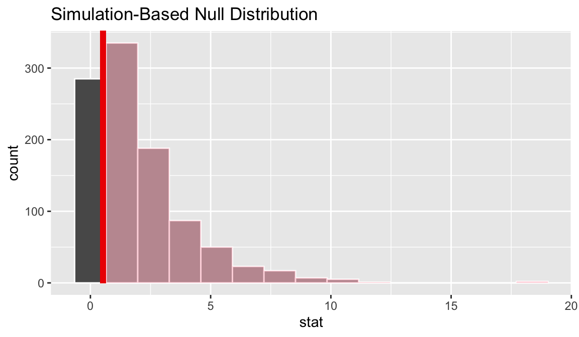
## # A tibble: 1 x 1
## p_value
## <dbl>
## 1 0.77One numerical variable, one categorical (2 levels) (diff in means)
Observed stat
( d_hat <- fli_small %>%
specify(dep_delay ~ season) %>%
calculate(stat = "diff in means", order = c("summer", "winter")) )## # A tibble: 1 x 1
## stat
## <dbl>
## 1 3null_distn <- fli_small %>%
specify(dep_delay ~ season) %>%
hypothesize(null = "independence") %>%
generate(reps = 1000, type = "permute") %>%
calculate(stat = "diff in means", order = c("summer", "winter"))
visualize(null_distn) +
  shade_p_value(obs_stat = d_hat, direction = "two_sided")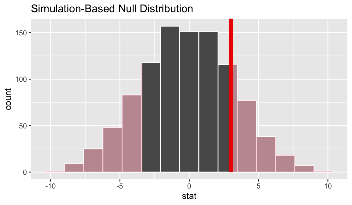
## # A tibble: 1 x 1
## p_value
## <dbl>
## 1 0.338One numerical variable, one categorical (2 levels) (t)
Standardized observed stat
( t_hat <- fli_small %>%
specify(dep_delay ~ season) %>%
calculate(stat = "t", order = c("summer", "winter")) )## # A tibble: 1 x 1
## stat
## <dbl>
## 1 0.891null_distn <- fli_small %>%
specify(dep_delay ~ season) %>%
hypothesize(null = "independence") %>%
generate(reps = 1000, type = "permute") %>%
calculate(stat = "t", order = c("summer", "winter"))
visualize(null_distn) +
shade_p_value(obs_stat = t_hat, direction = "two_sided")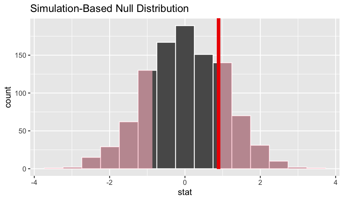
## # A tibble: 1 x 1
## p_value
## <dbl>
## 1 0.4Note the similarities in this plot and the previous one.
One numerical variable, one categorical (2 levels) (diff in medians)
Observed stat
( d_hat <- fli_small %>%
specify(dep_delay ~ season) %>%
calculate(stat = "diff in medians", order = c("summer", "winter")) )## # A tibble: 1 x 1
## stat
## <dbl>
## 1 1null_distn <- fli_small %>%
specify(dep_delay ~ season) %>% # alt: response = dep_delay,
# explanatory = season
hypothesize(null = "independence") %>%
generate(reps = 1000, type = "permute") %>%
calculate(stat = "diff in medians", order = c("summer", "winter"))
visualize(null_distn) +
shade_p_value(obs_stat = d_hat, direction = "two_sided")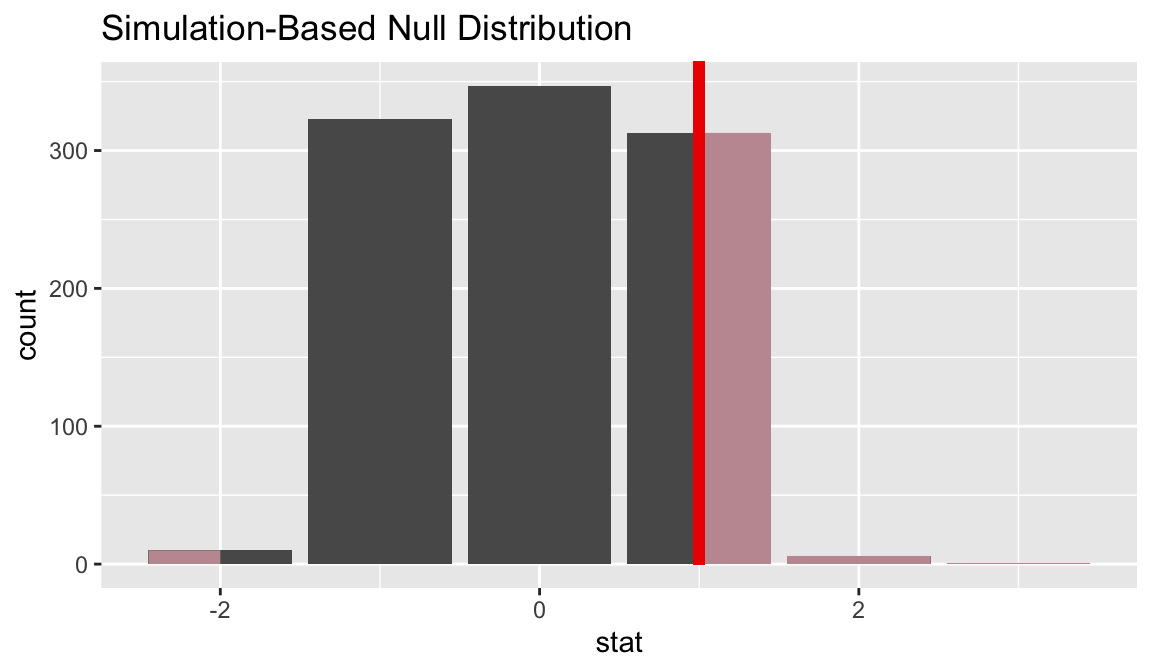
## # A tibble: 1 x 1
## p_value
## <dbl>
## 1 0.64One numerical, one categorical (>2 levels) - ANOVA
Observed stat
## # A tibble: 1 x 1
## stat
## <dbl>
## 1 0.686null_distn <- fli_small %>%
specify(arr_delay ~ origin) %>%
hypothesize(null = "independence") %>%
generate(reps = 1000, type = "permute") %>%
calculate(stat = "F")
visualize(null_distn) +
shade_p_value(obs_stat = F_hat, direction = "greater")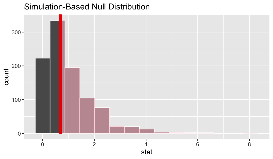
## # A tibble: 1 x 1
## p_value
## <dbl>
## 1 0.529Two numerical vars - SLR
Observed stat
## # A tibble: 1 x 1
## stat
## <dbl>
## 1 0.992null_distn <- fli_small %>%
specify(arr_delay ~ dep_delay) %>%
hypothesize(null = "independence") %>%
generate(reps = 1000, type = "permute") %>%
calculate(stat = "slope")
visualize(null_distn) +
shade_p_value(obs_stat = slope_hat, direction = "two_sided")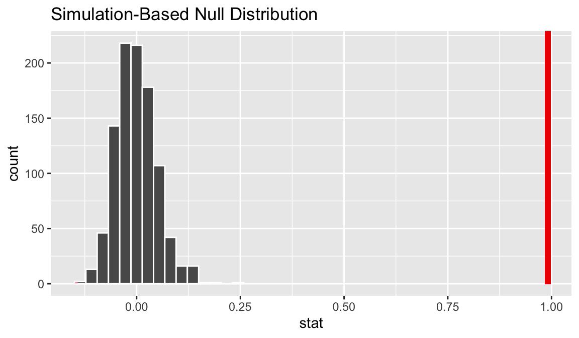
## # A tibble: 1 x 1
## p_value
## <dbl>
## 1 0Two numerical vars - correlation
Observed stat
( correlation_hat <- fli_small %>%
specify(arr_delay ~ dep_delay) %>%
calculate(stat = "correlation") )## # A tibble: 1 x 1
## stat
## <dbl>
## 1 0.895null_distn <- fli_small %>%
specify(arr_delay ~ dep_delay) %>%
hypothesize(null = "independence") %>%
generate(reps = 1000, type = "permute") %>%
calculate(stat = "correlation")
visualize(null_distn) +
shade_p_value(obs_stat = correlation_hat, direction = "two_sided")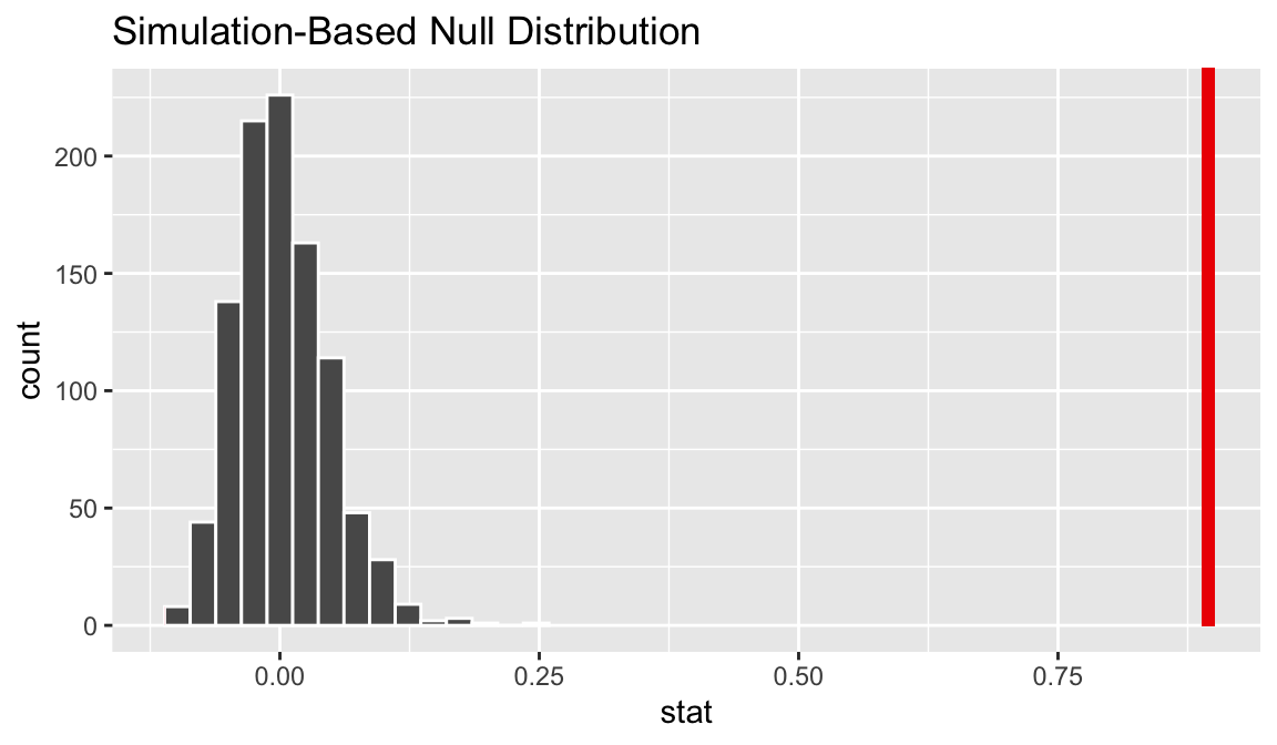
## # A tibble: 1 x 1
## p_value
## <dbl>
## 1 0Two numerical vars - SLR (t)
Not currently implemented since \(t\) could refer to standardized slope or standardized correlation.
Confidence intervals
One numerical (one mean)
Point estimate
## # A tibble: 1 x 1
## stat
## <dbl>
## 1 6.15boot <- fli_small %>%
specify(response = arr_delay) %>%
generate(reps = 1000, type = "bootstrap") %>%
calculate(stat = "mean")
( percentile_ci <- get_ci(boot) )## # A tibble: 1 x 2
## `2.5%` `97.5%`
## <dbl> <dbl>
## 1 2.61 9.60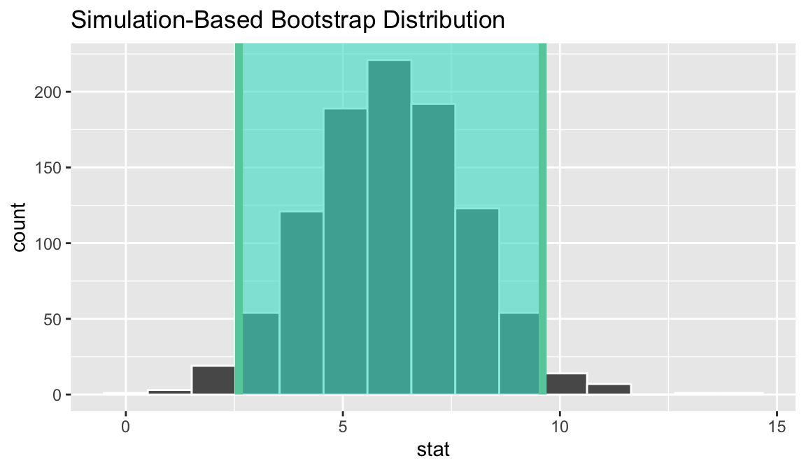
## # A tibble: 1 x 2
## lower upper
## <dbl> <dbl>
## 1 2.61 9.70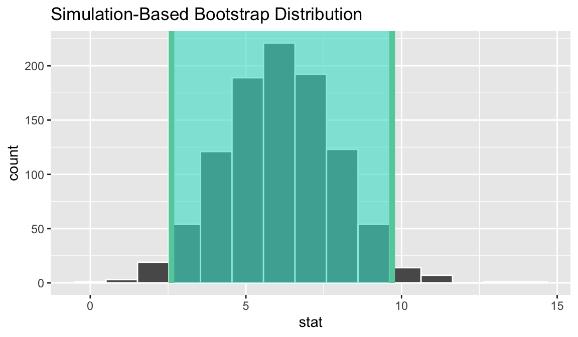
One numerical (one mean - standardized)
Point estimate
## # A tibble: 1 x 1
##    stat
##   <dbl>
## 1 3.30boot <- fli_small %>%
specify(response = arr_delay) %>%
generate(reps = 1000, type = "bootstrap") %>%
calculate(stat = "t")
( percentile_ci <- get_ci(boot) )## # A tibble: 1 x 2
## `2.5%` `97.5%`
## <dbl> <dbl>
## 1 1.62 4.88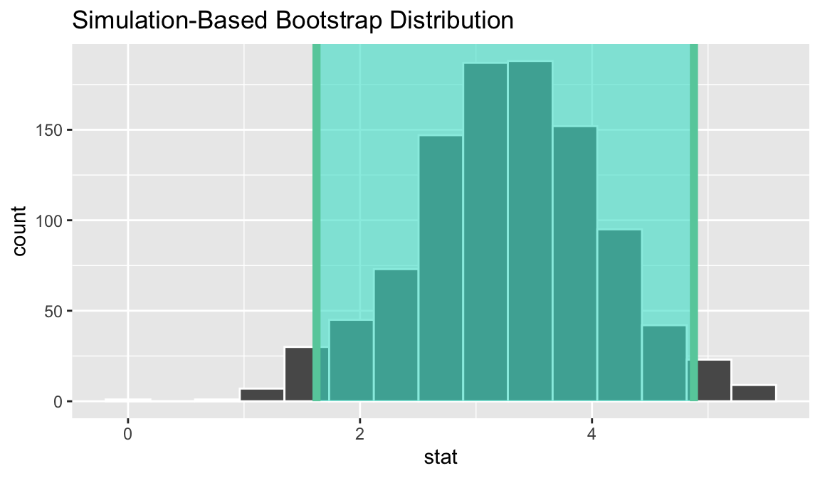
## # A tibble: 1 x 2
## lower upper
## <dbl> <dbl>
## 1 1.70 4.90
One categorical (one proportion)
Point estimate
( p_hat <- fli_small %>%
specify(response = day_hour, success = "morning") %>%
calculate(stat = "prop") )## # A tibble: 1 x 1
## stat
## <dbl>
## 1 0.452boot <- fli_small %>%
specify(response = day_hour, success = "morning") %>%
generate(reps = 1000, type = "bootstrap") %>%
calculate(stat = "prop")
( percentile_ci <- get_ci(boot) )## # A tibble: 1 x 2
## `2.5%` `97.5%`
## <dbl> <dbl>
## 1 0.406 0.496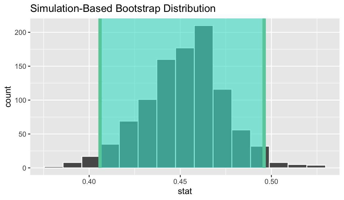
## # A tibble: 1 x 2
## lower upper
## <dbl> <dbl>
## 1 0.408 0.496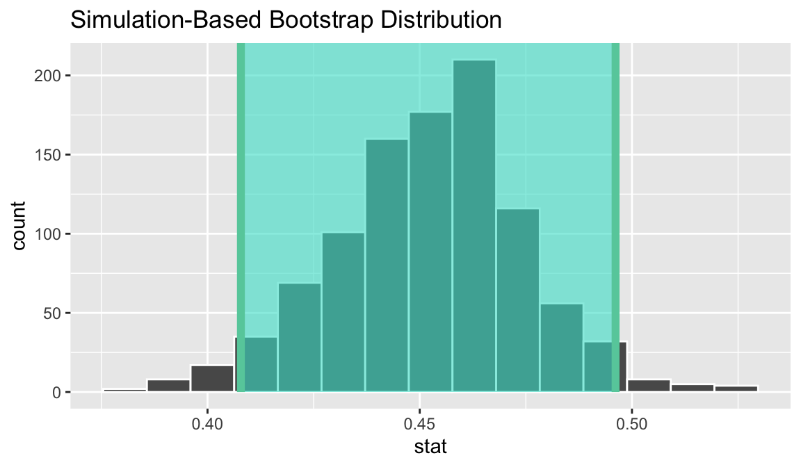
One numerical variable, one categorical (2 levels) (diff in means)
Point estimate
( d_hat <- fli_small %>%
specify(arr_delay ~ season) %>%
calculate(stat = "diff in means", order = c("summer", "winter")) )## # A tibble: 1 x 1
## stat
## <dbl>
## 1 5.63boot <- fli_small %>%
specify(arr_delay ~ season) %>%
generate(reps = 1000, type = "bootstrap") %>%
calculate(stat = "diff in means", order = c("summer", "winter"))
( percentile_ci <- get_ci(boot) )## # A tibble: 1 x 2
## `2.5%` `97.5%`
## <dbl> <dbl>
## 1 -2.03 12.5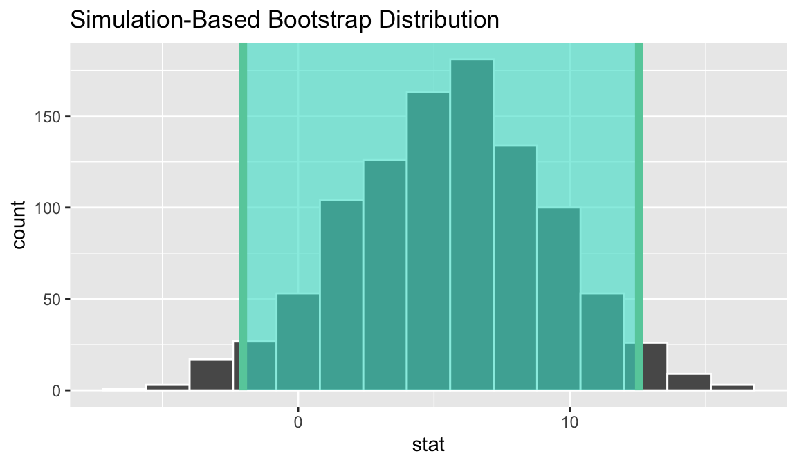
## # A tibble: 1 x 2
## lower upper
## <dbl> <dbl>
## 1 -1.61 12.9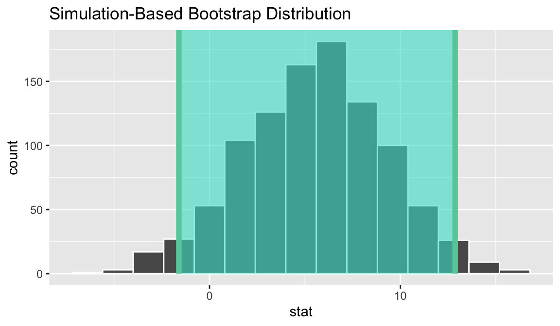
One numerical variable, one categorical (2 levels) (t)
Standardized point estimate
( t_hat <- fli_small %>%
specify(arr_delay ~ season) %>%
calculate(stat = "t", order = c("summer", "winter")) )## # A tibble: 1 x 1
## stat
## <dbl>
## 1 1.51boot <- fli_small %>%
specify(arr_delay ~ season) %>%
generate(reps = 1000, type = "bootstrap") %>%
calculate(stat = "t", order = c("summer", "winter"))
( percentile_ci <- get_ci(boot) )## # A tibble: 1 x 2
## `2.5%` `97.5%`
## <dbl> <dbl>
## 1 -0.359 3.74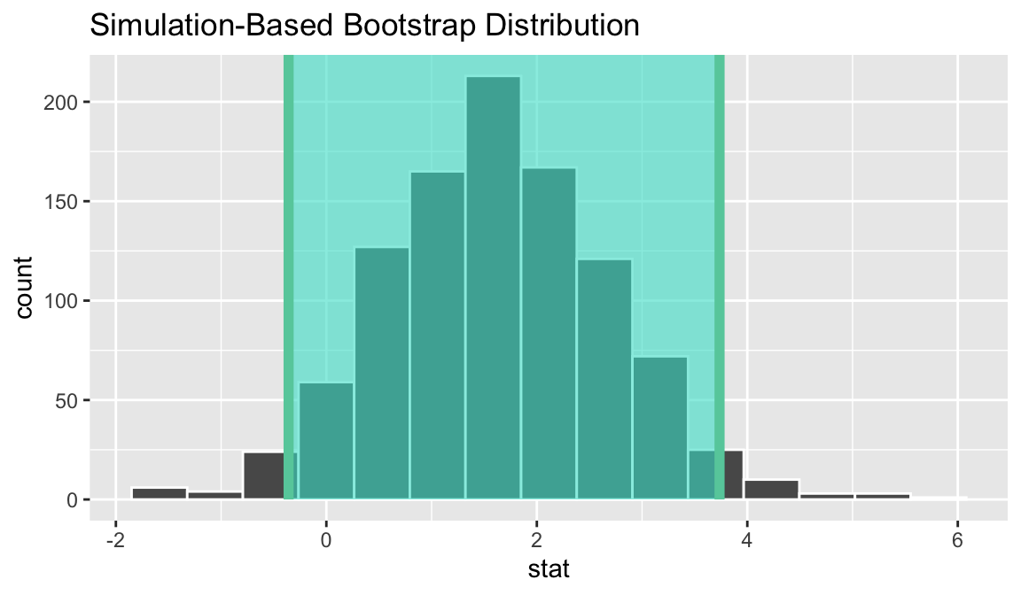
## # A tibble: 1 x 2
## lower upper
## <dbl> <dbl>
## 1 -0.578 3.60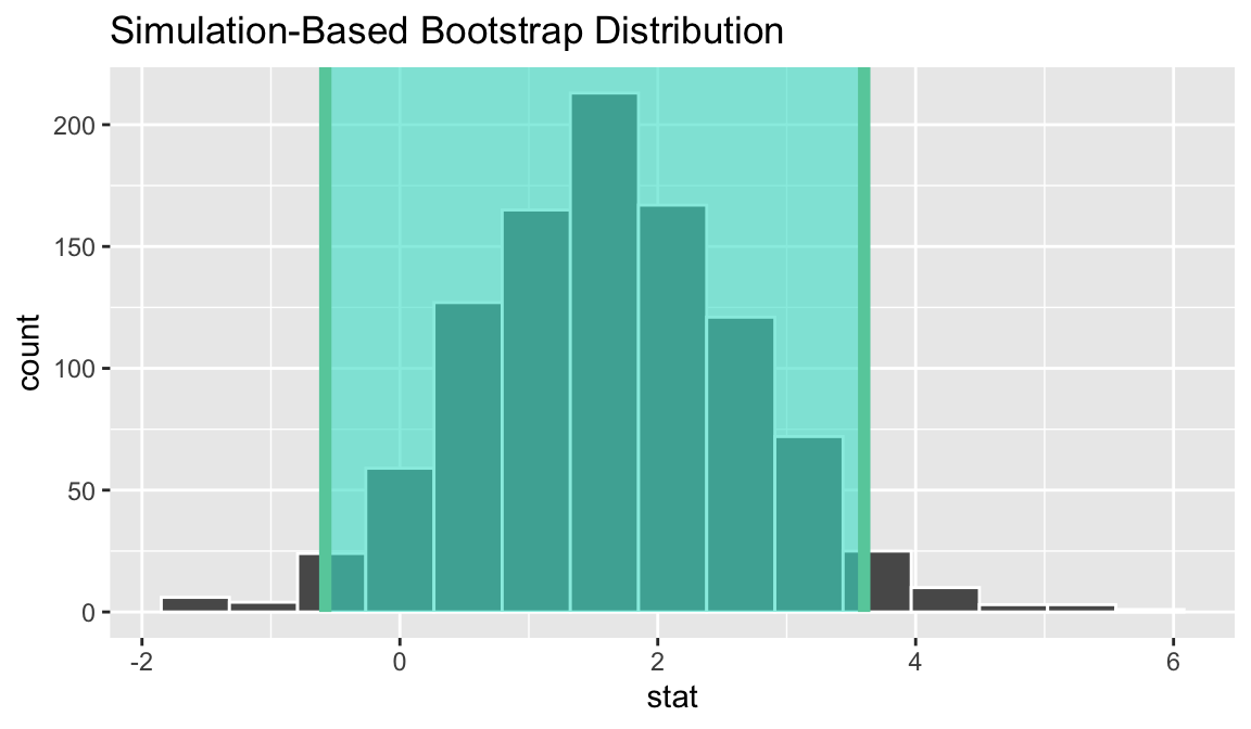
Two categorical variables (diff in proportions)
Point estimate
( d_hat <- fli_small %>%
specify(day_hour ~ season, success = "morning") %>%
calculate(stat = "diff in props", order = c("summer", "winter")) )## # A tibble: 1 x 1
## stat
## <dbl>
## 1 -0.00438boot <- fli_small %>%
specify(day_hour ~ season, success = "morning") %>%
generate(reps = 1000, type = "bootstrap") %>%
calculate(stat = "diff in props", order = c("summer", "winter"))
( percentile_ci <- get_ci(boot) )## # A tibble: 1 x 2
## `2.5%` `97.5%`
## <dbl> <dbl>
## 1 -0.0957 0.0818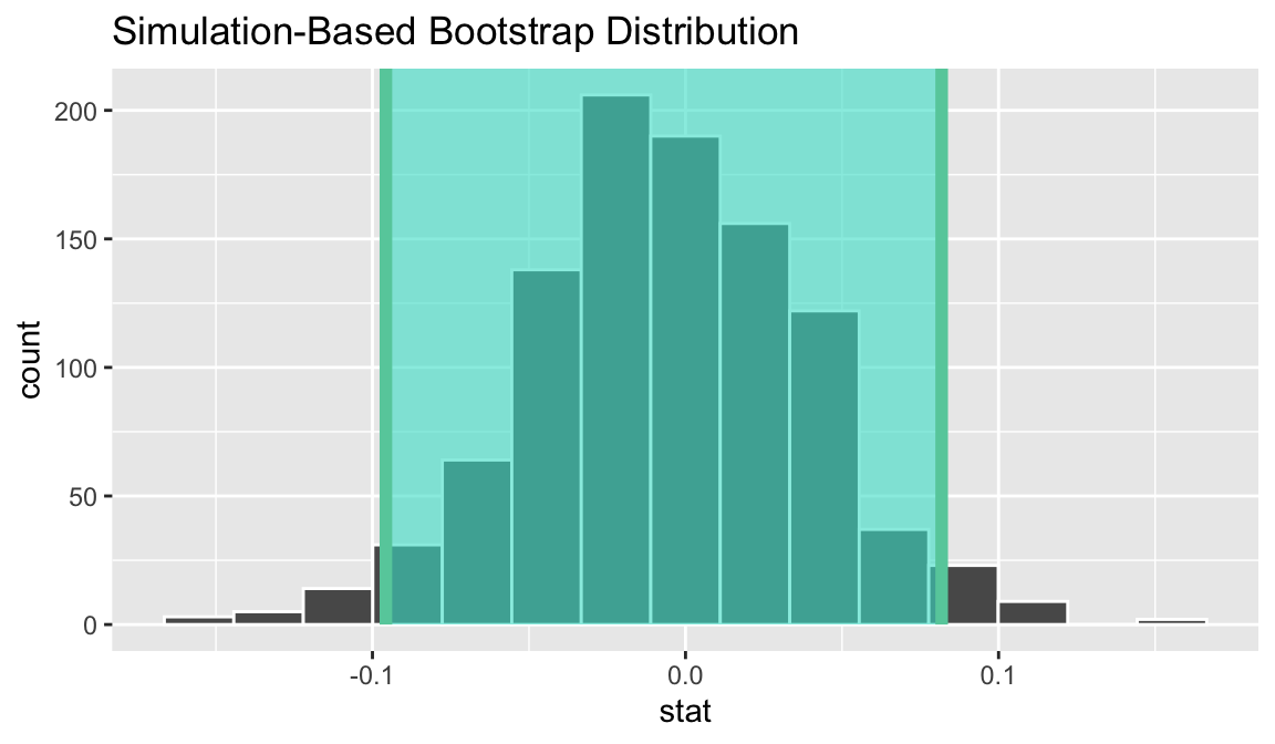
## # A tibble: 1 x 2
## lower upper
## <dbl> <dbl>
## 1 -0.0914 0.0826
Two categorical variables (z)
Standardized point estimate
( z_hat <- fli_small %>%
specify(day_hour ~ season, success = "morning") %>%
calculate(stat = "z", order = c("summer", "winter")) )## # A tibble: 1 x 1
## stat
## <dbl>
## 1 -0.0985boot <- fli_small %>%
specify(day_hour ~ season, success = "morning") %>%
generate(reps = 1000, type = "bootstrap") %>%
calculate(stat = "z", order = c("summer", "winter"))
( percentile_ci <- get_ci(boot) )## # A tibble: 1 x 2
## `2.5%` `97.5%`
## <dbl> <dbl>
## 1 -1.96 1.79
## # A tibble: 1 x 2
## lower upper
## <dbl> <dbl>
## 1 -2.04 1.85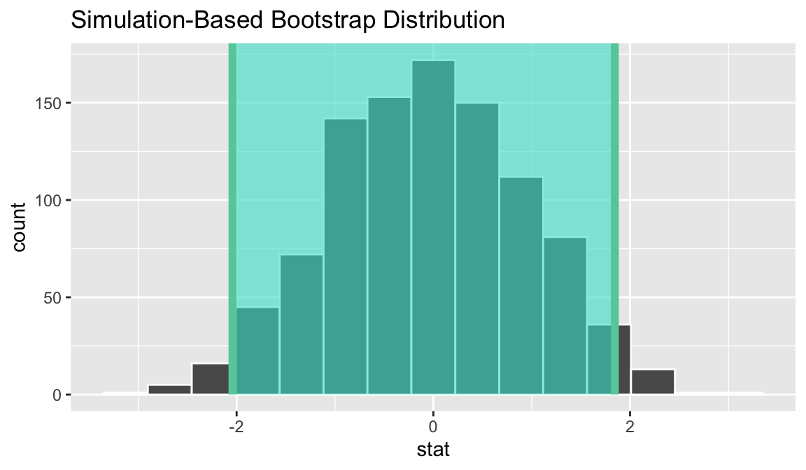
Two numerical vars - SLR
Point estimate
## # A tibble: 1 x 1
##    stat
##   <dbl>
## 1 0.992boot <- fli_small %>%
specify(arr_delay ~ dep_delay) %>%
generate(reps = 1000, type = "bootstrap") %>%
calculate(stat = "slope")
( percentile_ci <- get_ci(boot) )## # A tibble: 1 x 2
## `2.5%` `97.5%`
## <dbl> <dbl>
## 1 0.946 1.03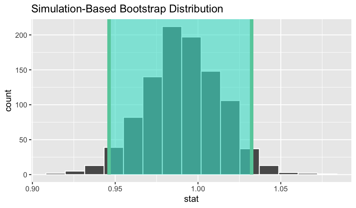
## # A tibble: 1 x 2
## lower upper
## <dbl> <dbl>
## 1 0.947 1.04
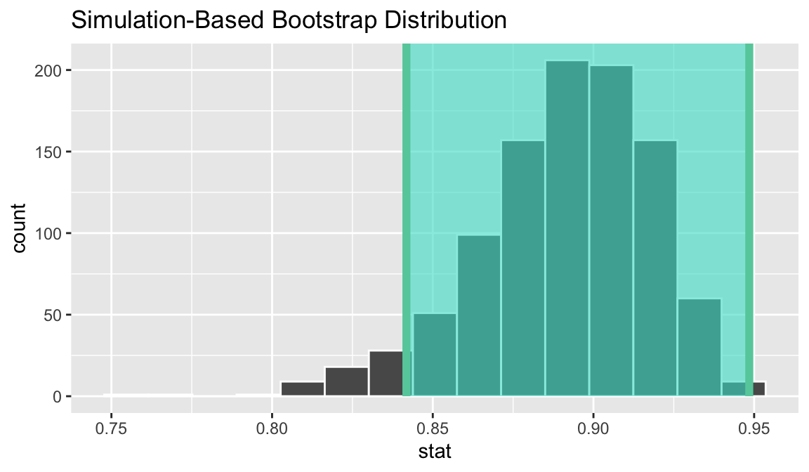
Two numerical vars - correlation
Point estimate
( correlation_hat <- fli_small %>%
  specify(arr_delay ~ dep_delay) %>%
  calculate(stat = "correlation") )
## # A tibble: 1 x 1
## stat
## <dbl>
## 1 0.895boot <- fli_small %>%
specify(arr_delay ~ dep_delay) %>%
generate(reps = 1000, type = "bootstrap") %>%
calculate(stat = "correlation")
( percentile_ci <- get_ci(boot) )## # A tibble: 1 x 2
## `2.5%` `97.5%`
## <dbl> <dbl>
## 1 0.827 0.933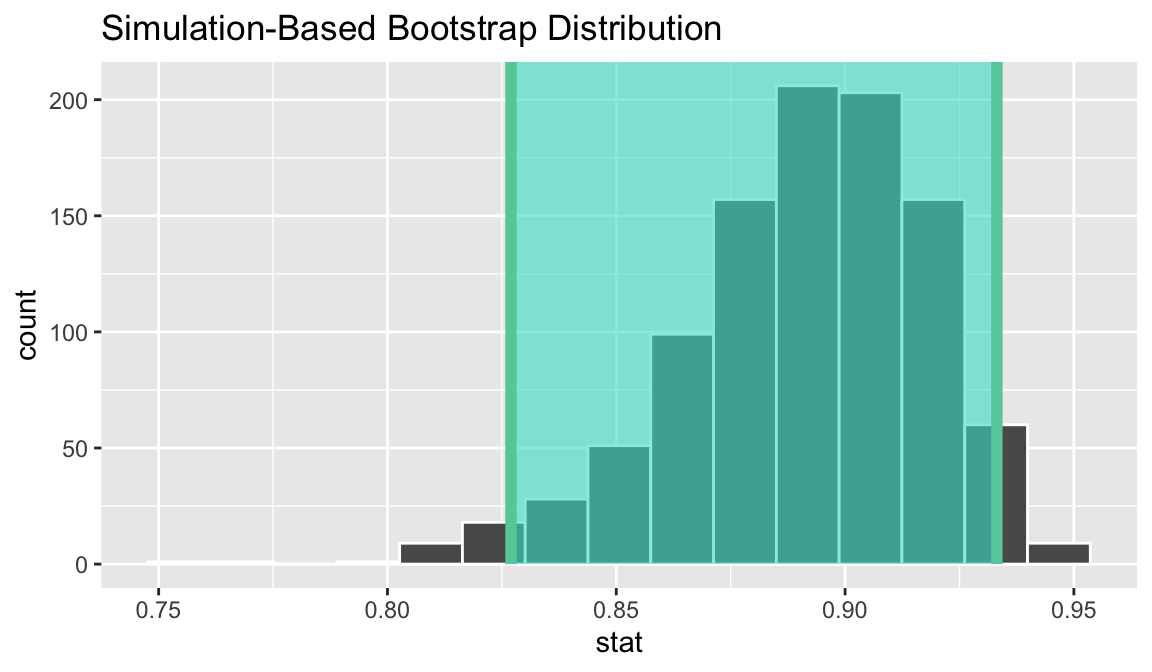
## # A tibble: 1 x 2
##   lower upper
##   <dbl> <dbl>
## 1 0.842 0.948