Two sample \(t\) test example using nycflights13 flights data

Chester Ismay

2019-11-19

Note: The type argument in generate() is automatically filled based on the entries for specify() and hypothesize(). It can be removed throughout the examples that follow. It is left in to reiterate the type of generation process being performed.

Data preparation

library(nycflights13)
library(dplyr)
library(stringr)
library(infer)
set.seed(2017)
fli_small <- flights %>% 
  sample_n(size = 500) %>% 
  mutate(half_year = case_when(
    between(month, 1, 6) ~ "h1",
    between(month, 7, 12) ~ "h2"
  )) %>% 
  mutate(day_hour = case_when(
    between(hour, 1, 12) ~ "morning",
    between(hour, 13, 24) ~ "not morning"
  )) %>% 
  select(arr_delay, dep_delay, half_year, 
         day_hour, origin, carrier)

• Two numeric - arr_delay, dep_delay
• Two categories
  • half_year ("h1", "h2"),
  • day_hour ("morning", "not morning")
• Three categories - origin ("EWR", "JFK", "LGA")
• Sixteen categories - carrier

---

One numerical variable, one categorical (2 levels)

Calculate observed statistic

The recommended approach is to use specify() %>% calculate():

obs_t <- fli_small %>%
  specify(arr_delay ~ half_year) %>%
  calculate(stat = "t", order = c("h1", "h2"))

## Warning: Removed 9 rows containing missing values.

The observed \(t\) statistic is 0.2765533.

Or using t_test in infer

obs_t <- fli_small %>% 
  t_test(formula = arr_delay ~ half_year, alternative = "two_sided",
         order = c("h1", "h2")) %>% 
  dplyr::pull(statistic)

The observed \(t\) statistic is 0.2765533.

Or using another shortcut function in infer:

obs_t <- fli_small %>% 
  t_stat(formula = arr_delay ~ half_year, order = c("h1", "h2"))

The observed \(t\) statistic is 0.2765533.

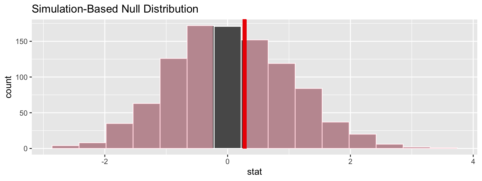
Randomization approach to t-statistic

t_null_perm <- fli_small %>%
  # alt: response = arr_delay, explanatory = half_year
  specify(arr_delay ~ half_year) %>%
  hypothesize(null = "independence") %>%
  generate(reps = 1000, type = "permute") %>%
  calculate(stat = "t", order = c("h1", "h2"))

## Warning: Removed 9 rows containing missing values.

visualize(t_null_perm) +
  shade_p_value(obs_stat = obs_t, direction = "two_sided")

Calculate the randomization-based \(p\)-value

t_null_perm %>% 
  get_p_value(obs_stat = obs_t, direction = "two_sided")

## # A tibble: 1 x 1
##   p_value
##     <dbl>
## 1   0.806

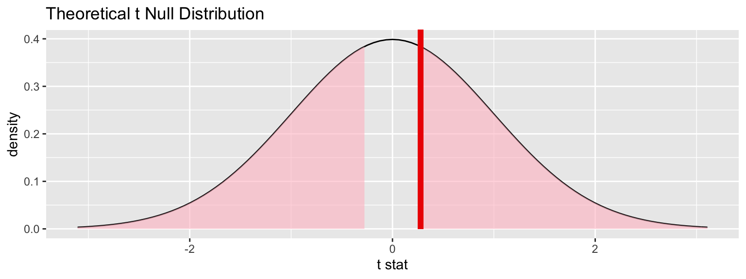
Theoretical distribution

t_null_theor <- fli_small %>%
  # alt: response = arr_delay, explanatory = half_year
  specify(arr_delay ~ half_year) %>%
  hypothesize(null = "independence") %>%
  # generate() ## Not used for theoretical
  calculate(stat = "t", order = c("h1", "h2"))

## Warning: Removed 9 rows containing missing values.

visualize(t_null_theor, method = "theoretical") +
  shade_p_value(obs_stat = obs_t, direction = "two_sided")

## Warning: Check to make sure the conditions have been met for the
## theoretical method. {infer} currently does not check these for you.

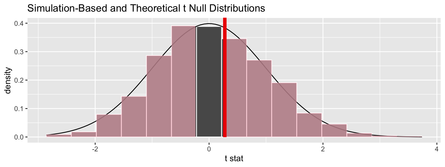
Overlay appropriate \(t\) distribution on top of permuted t-statistics

visualize(t_null_perm, method = "both") +
  shade_p_value(obs_stat = obs_t, direction = "two_sided")

## Warning: Check to make sure the conditions have been met for the
## theoretical method. {infer} currently does not check these for you.

Compute theoretical p-value

fli_small %>% 
  t_test(formula = arr_delay ~ half_year,
         alternative = "two_sided",
         order = c("h1", "h2")) %>% 
  dplyr::pull(p_value)

## [1] 0.7822402