Note: The type argument in generate() is automatically filled based on the entries for specify() and hypothesize(). It can be removed throughout the examples that follow. It is left in to reiterate the type of generation process being performed.

This vignette is designed to show how to use the {infer} package with {dplyr} syntax. It does not show how to calculate observed statistics or p-values using the {infer} package. To see examples of these, check out the “Computation of observed statistics…” vignette instead.

Data preparation

library(nycflights13)
library(dplyr)
library(ggplot2)
library(stringr)
library(infer)
set.seed(2017)
fli_small <- flights %>% 
  na.omit() %>%
  sample_n(size = 500) %>% 
  mutate(season = case_when(
    month %in% c(10:12, 1:3) ~ "winter",
    month %in% c(4:9) ~ "summer"
  )) %>% 
  mutate(day_hour = case_when(
    between(hour, 1, 12) ~ "morning",
    between(hour, 13, 24) ~ "not morning"
  )) %>% 
  select(arr_delay, dep_delay, season, 
         day_hour, origin, carrier)

Two numeric - arr_delay, dep_delay
Two categories
- season ("winter", "summer"),
- day_hour ("morning", "not morning")
Three categories - origin ("EWR", "JFK", "LGA")
Sixteen categories - carrier

Hypothesis tests

One numerical variable (mean)

x_bar <- fli_small %>%
  summarize(mean(dep_delay)) %>%
  pull()

null_distn <- fli_small %>%
  specify(response = dep_delay) %>%
  hypothesize(null = "point", mu = 10) %>%
  generate(reps = 1000, type = "bootstrap") %>%
  calculate(stat = "mean")
ggplot(data = null_distn, mapping = aes(x = stat)) +
  geom_density() +
  geom_vline(xintercept = x_bar, color = "red")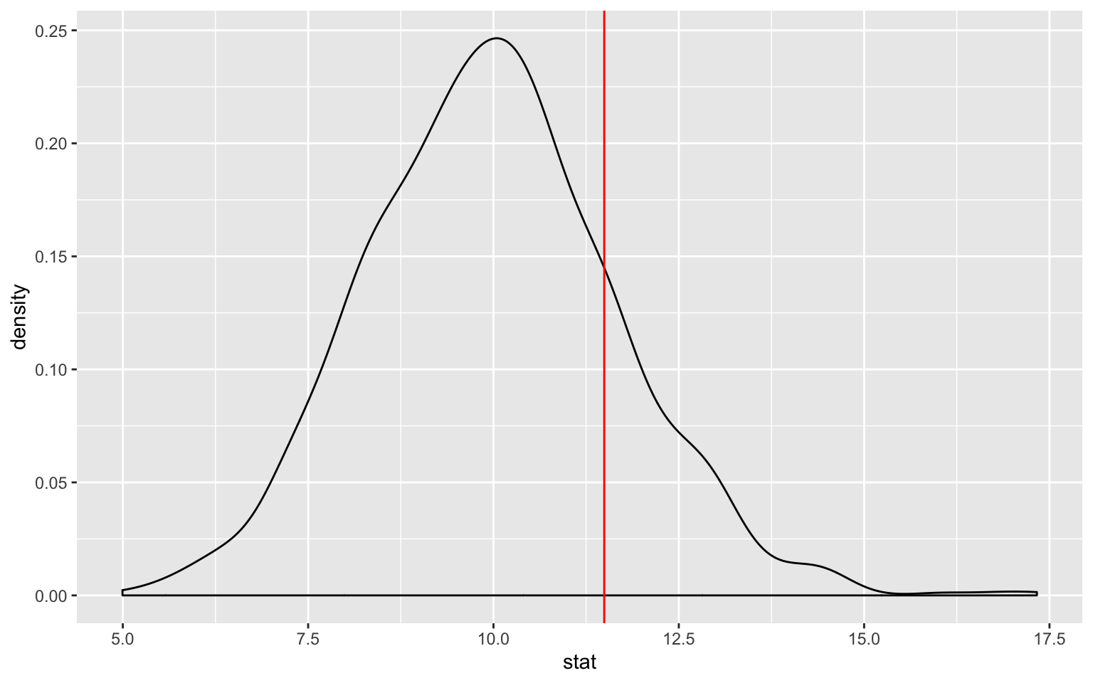

null_distn %>%
  summarize(p_value = mean(stat >= x_bar) * 2)

## # A tibble: 1 x 1
##   p_value
##     <dbl>
## 1   0.356

One numerical variable (median)

x_tilde <- fli_small %>%
  summarize(median(dep_delay)) %>%
  pull()
null_distn <- fli_small %>%
  specify(response = dep_delay) %>%
  hypothesize(null = "point", med = -1) %>% 
  generate(reps = 1000, type = "bootstrap") %>% 
  calculate(stat = "median")
ggplot(null_distn, aes(x = stat)) +
  geom_bar() +
  geom_vline(xintercept = x_tilde, color = "red")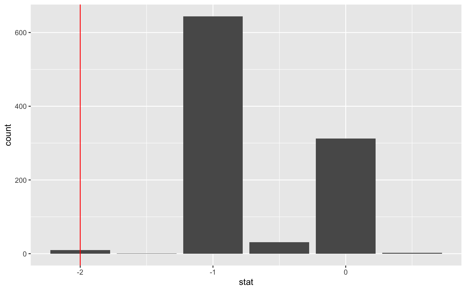

null_distn %>%
  summarize(p_value = mean(stat <= x_tilde) * 2)

## # A tibble: 1 x 1
##   p_value
##     <dbl>
## 1    0.02

One categorical (one proportion)

p_hat <- fli_small %>%
  summarize(mean(day_hour == "morning")) %>%
  pull()
null_distn <- fli_small %>%
  specify(response = day_hour, success = "morning") %>%
  hypothesize(null = "point", p = .5) %>%
  generate(reps = 1000, type = "simulate") %>%
  calculate(stat = "prop")
ggplot(null_distn, aes(x = stat)) +
  geom_bar() +
  geom_vline(xintercept = p_hat, color = "red")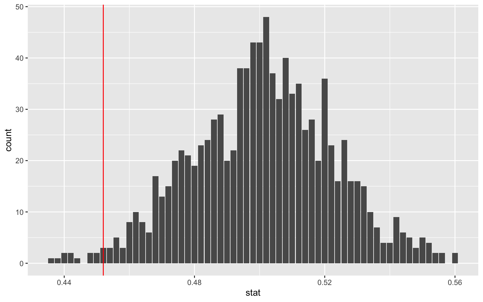

null_distn %>%
  summarize(p_value = mean(stat <= p_hat) * 2)

## # A tibble: 1 x 1
##   p_value
##     <dbl>
## 1   0.028

Logical variables will be coerced to factors:

null_distn <- fli_small %>%
  mutate(day_hour_logical = (day_hour == "morning")) %>%
  specify(response = day_hour_logical, success = "TRUE") %>%
  hypothesize(null = "point", p = .5) %>%
  generate(reps = 1000, type = "simulate") %>%
  calculate(stat = "prop")

Two categorical (2 level) variables

d_hat <- fli_small %>%
  group_by(season) %>%
  summarize(prop = mean(day_hour == "morning")) %>%
  summarize(diff(prop)) %>%
  pull()
null_distn <- fli_small %>%
  specify(day_hour ~ season, success = "morning") %>%
  hypothesize(null = "independence") %>% 
  generate(reps = 1000, type = "permute") %>% 
  calculate(stat = "diff in props", order = c("winter", "summer"))
ggplot(null_distn, aes(x = stat)) +
  geom_density() +
  geom_vline(xintercept = d_hat, color = "red")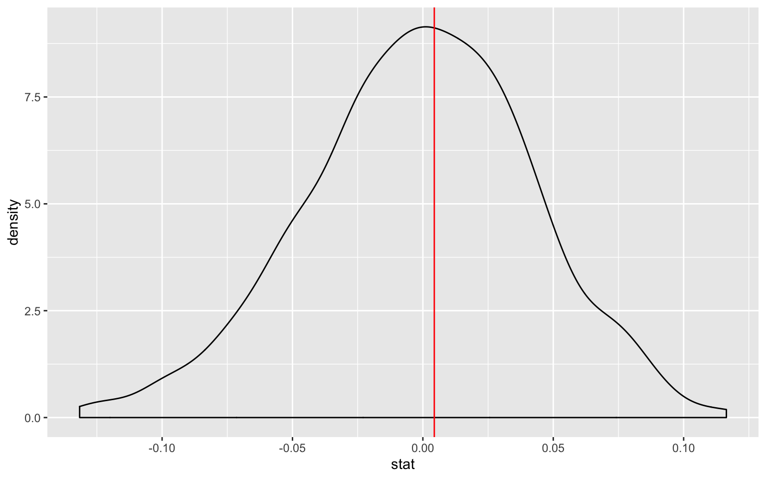

null_distn %>%
  summarize(p_value = mean(stat <= d_hat) * 2) %>%
  pull()

## [1] 1.158

One categorical (>2 level) - GoF

Chisq_hat <- fli_small %>%
  specify(response = origin) %>%
  hypothesize(null = "point", 
              p = c("EWR" = .33, "JFK" = .33, "LGA" = .34)) %>% 
  calculate(stat = "Chisq")
null_distn <- fli_small %>%
  specify(response = origin) %>%
  hypothesize(null = "point", 
              p = c("EWR" = .33, "JFK" = .33, "LGA" = .34)) %>% 
  generate(reps = 1000, type = "simulate") %>% 
  calculate(stat = "Chisq")
ggplot(null_distn, aes(x = stat)) +
  geom_density() +
  geom_vline(xintercept = pull(Chisq_hat), color = "red")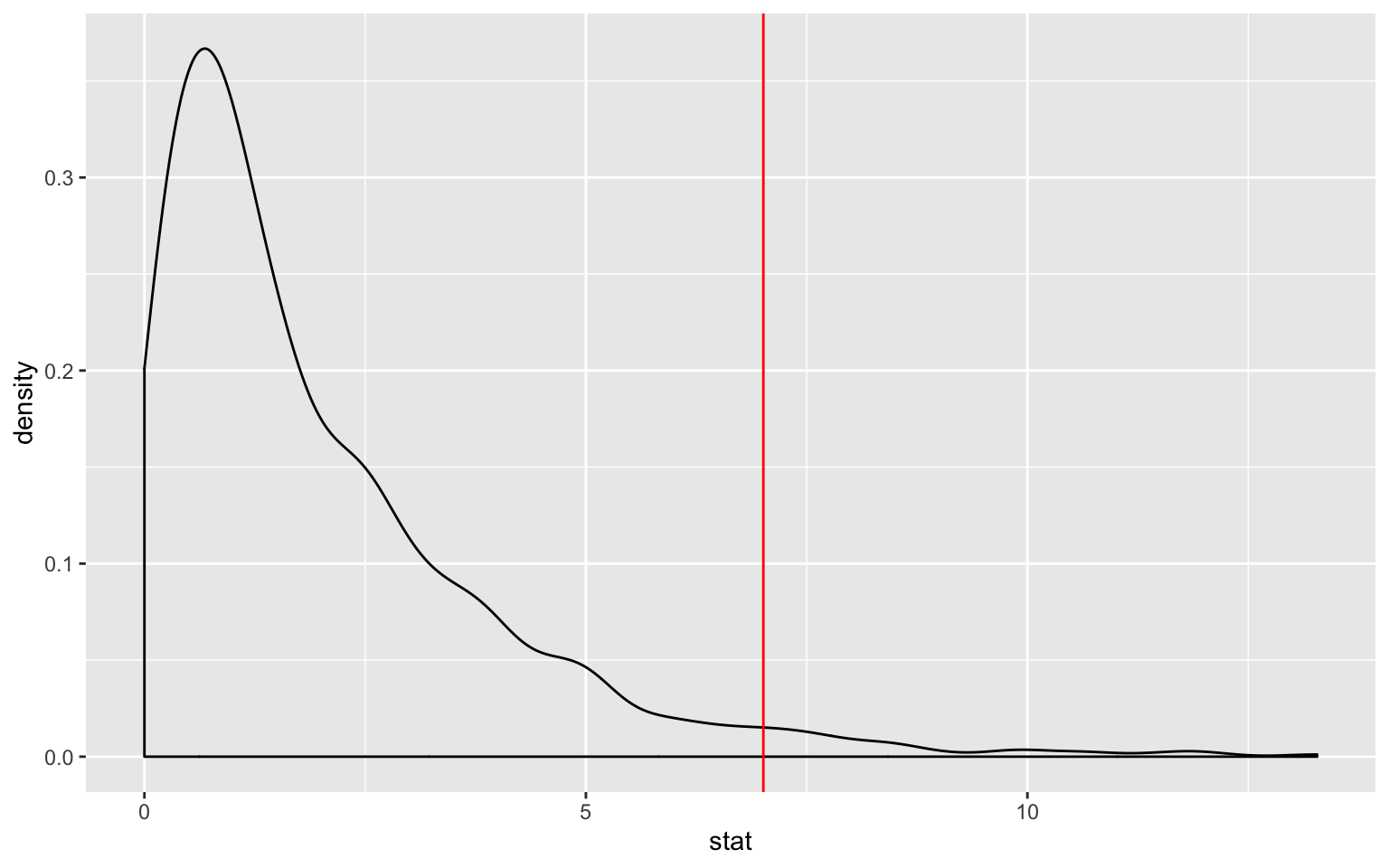

null_distn %>%
  summarize(p_value = mean(stat >= pull(Chisq_hat))) %>%
  pull()

## [1] 0.03

Two categorical (>2 level) variables

Chisq_hat <- fli_small %>%
  chisq_stat(formula = day_hour ~ origin)
null_distn <- fli_small %>%
  specify(day_hour ~ origin, success = "morning") %>%
  hypothesize(null = "independence") %>% 
  generate(reps = 1000, type = "permute") %>% 
  calculate(stat = "Chisq")
ggplot(null_distn, aes(x = stat)) +
  geom_density() +
  geom_vline(xintercept = Chisq_hat, color = "red")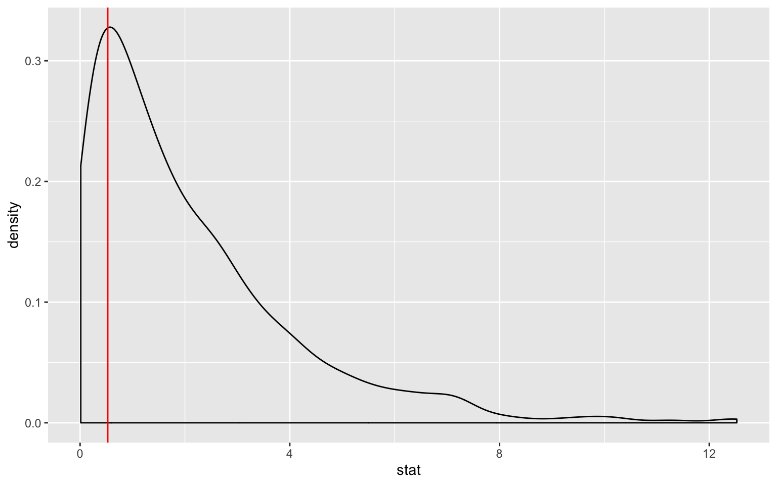

null_distn %>%
  summarize(p_value = mean(stat >= Chisq_hat)) %>%
  pull()

## [1] 0.777

One numerical variable, one categorical (2 levels) (diff in means)

d_hat <- fli_small %>% 
  group_by(season) %>% 
  summarize(mean_stat = mean(dep_delay)) %>% 
  # Since summer - winter
  summarize(-diff(mean_stat)) %>% 
  pull()
null_distn <- fli_small %>%
  specify(dep_delay ~ season) %>% # alt: response = dep_delay, 
  # explanatory = season
  hypothesize(null = "independence") %>%
  generate(reps = 1000, type = "permute") %>%
  calculate(stat = "diff in means", order = c("summer", "winter"))
ggplot(null_distn, aes(x = stat)) +
  geom_density() +
  geom_vline(xintercept = d_hat, color = "red")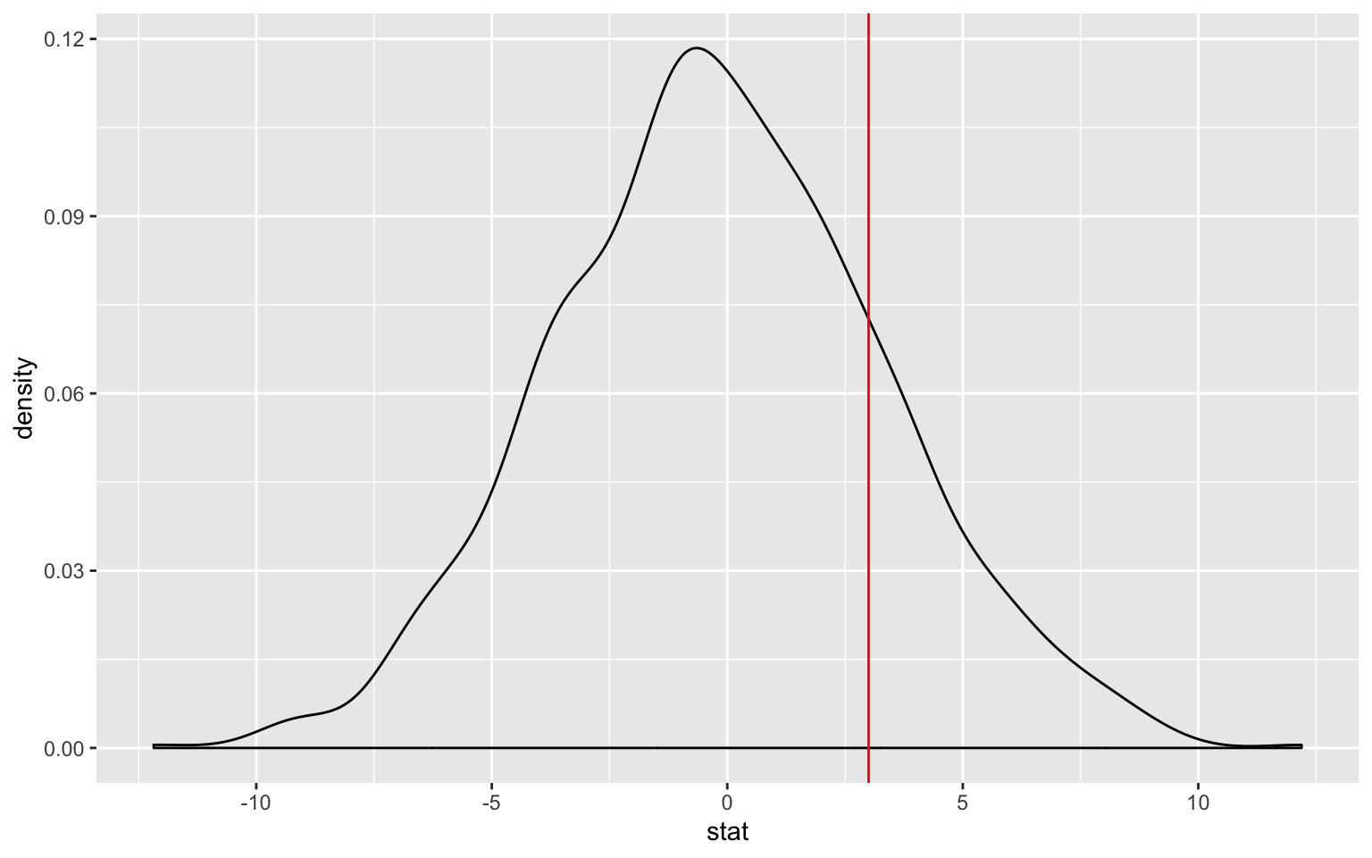

null_distn %>%
  summarize(p_value = mean(stat <= d_hat) * 2) %>%
  pull()

## [1] 1.638

One numerical variable, one categorical (2 levels) (diff in medians)

d_hat <- fli_small %>% 
  group_by(season) %>% 
  summarize(median_stat = median(dep_delay)) %>% 
  # Since summer - winter
  summarize(-diff(median_stat)) %>% 
  pull()
null_distn <- fli_small %>%
  specify(dep_delay ~ season) %>% # alt: response = dep_delay, 
  # explanatory = season
  hypothesize(null = "independence") %>%
  generate(reps = 1000, type = "permute") %>%
  calculate(stat = "diff in medians", order = c("summer", "winter"))
ggplot(null_distn, aes(x = stat)) +
  geom_bar() +
  geom_vline(xintercept = d_hat, color = "red")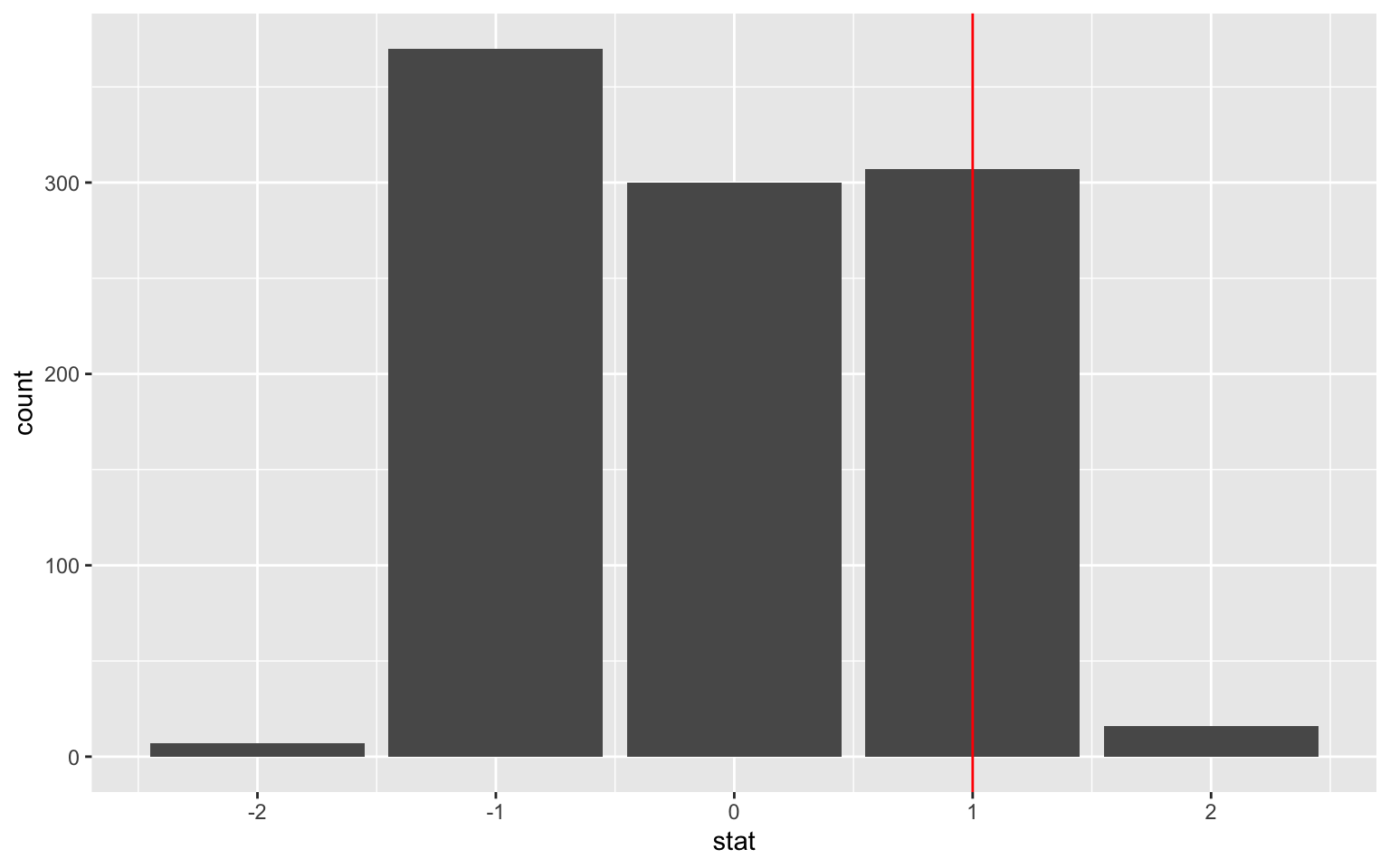

null_distn %>%
  summarize(p_value = mean(stat >= d_hat) * 2) %>%
  pull()

## [1] 0.646

One numerical, one categorical (>2 levels) - ANOVA

F_hat <- anova(
               aov(formula = arr_delay ~ origin, data = fli_small)
               )$`F value`[1]
null_distn <- fli_small %>%
   specify(arr_delay ~ origin) %>% # alt: response = arr_delay, 
   # explanatory = origin
   hypothesize(null = "independence") %>%
   generate(reps = 1000, type = "permute") %>%
   calculate(stat = "F")
ggplot(null_distn, aes(x = stat)) +
  geom_density() +
  geom_vline(xintercept = F_hat, color = "red")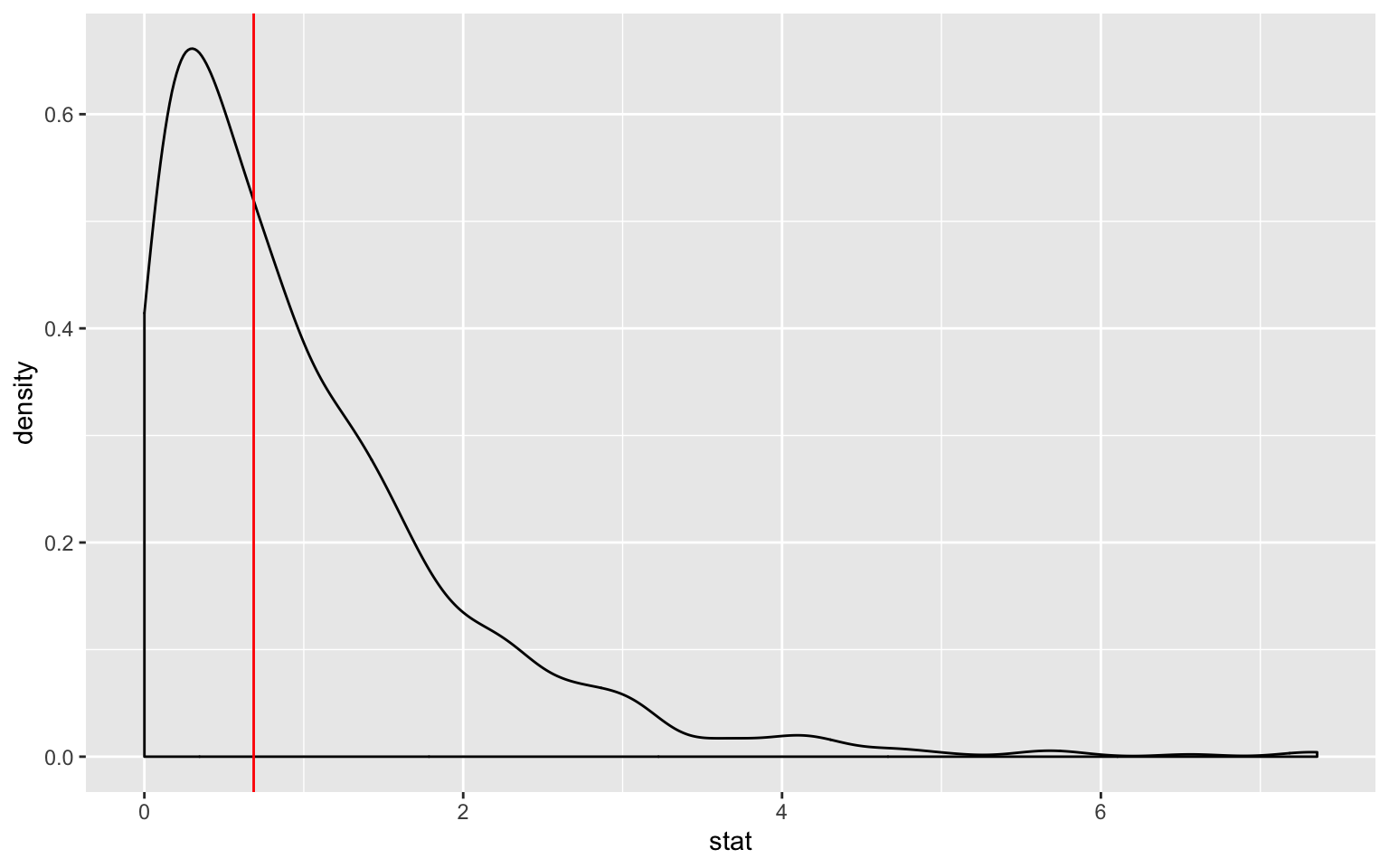

null_distn %>% 
  summarize(p_value = mean(stat >= F_hat)) %>%
  pull()

## [1] 0.526

Two numerical vars - SLR

slope_hat <- lm(arr_delay ~ dep_delay, data = fli_small) %>% 
  broom::tidy() %>% 
  filter(term == "dep_delay") %>% 
  pull(estimate)
null_distn <- fli_small %>%
   specify(arr_delay ~ dep_delay) %>% 
   hypothesize(null = "independence") %>%
   generate(reps = 1000, type = "permute") %>%
   calculate(stat = "slope")
ggplot(null_distn, aes(x = stat)) +
  geom_density() +
  geom_vline(xintercept = slope_hat, color = "red")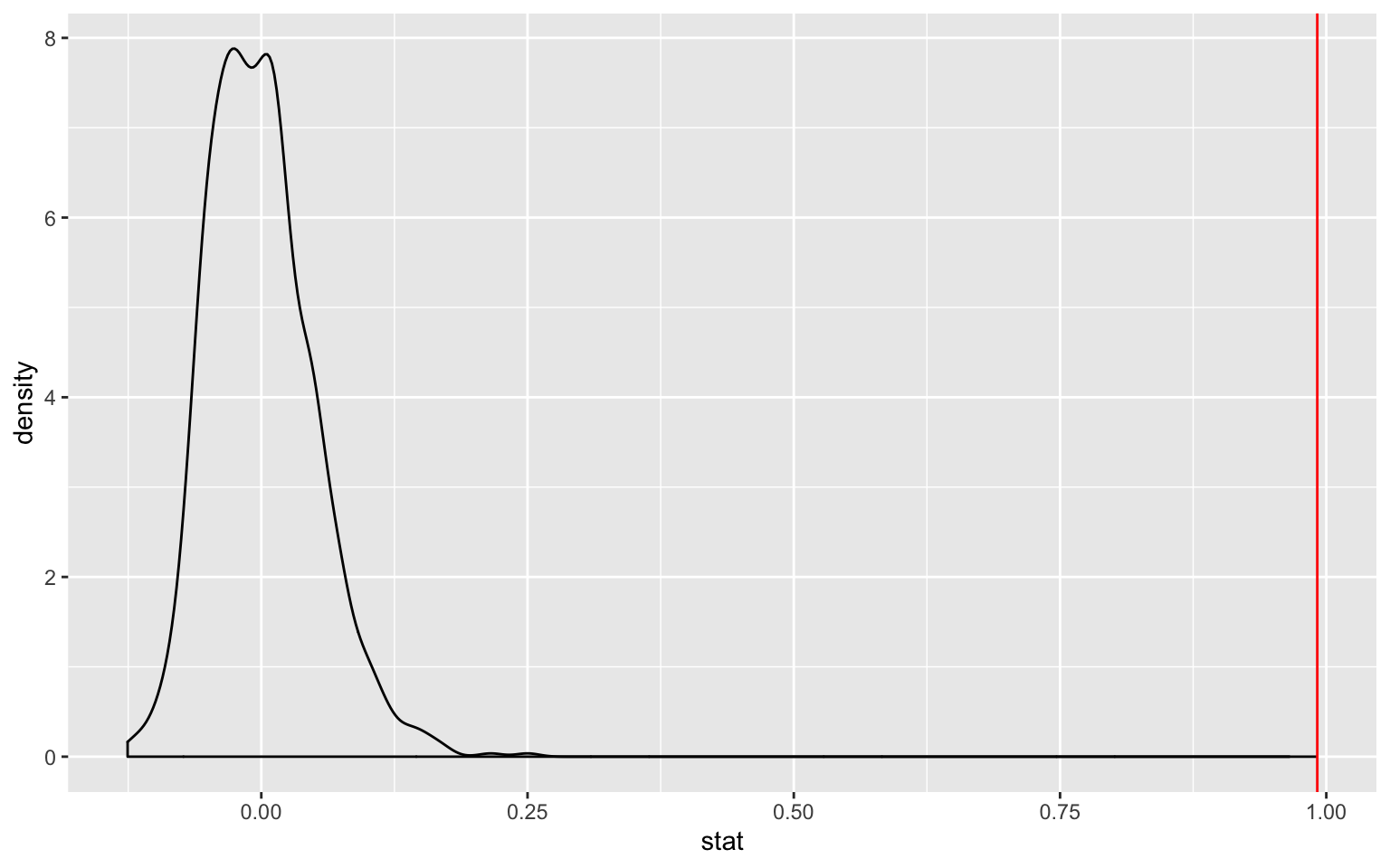

null_distn %>% 
  summarize(p_value = mean(stat >= slope_hat) * 2) %>%
  pull()

## [1] 0

Confidence intervals

One numerical (one mean)

x_bar <- fli_small %>%
   summarize(mean(arr_delay)) %>%
   pull()
boot <- fli_small %>%
   specify(response = arr_delay) %>%
   generate(reps = 1000, type = "bootstrap") %>%
   calculate(stat = "mean") %>%
   pull()
c(lower = x_bar - 2 * sd(boot),
  upper = x_bar + 2 * sd(boot))

##    lower    upper 
## 2.504552 9.803448

One categorical (one proportion)

p_hat <- fli_small %>%
 summarize(mean(day_hour == "morning")) %>%
 pull()
boot <- fli_small %>%
 specify(response = day_hour, success = "morning") %>%
 generate(reps = 1000, type = "bootstrap") %>%
 calculate(stat = "prop") %>%
 pull()
c(lower = p_hat - 2 * sd(boot),
 upper = p_hat + 2 * sd(boot))

##     lower     upper 
## 0.4085618 0.4954382

One numerical variable, one categorical (2 levels) (diff in means)

d_hat <- fli_small %>% 
  group_by(season) %>% 
  summarize(mean_stat = mean(arr_delay)) %>% 
  # Since summer - winter
  summarize(-diff(mean_stat)) %>% 
  pull()
boot <- fli_small %>%
   specify(arr_delay ~ season) %>%
   generate(reps = 1000, type = "bootstrap") %>%
   calculate(stat = "diff in means", order = c("summer", "winter")) %>% 
   pull()
c(lower = d_hat - 2 * sd(boot), 
  upper = d_hat + 2 * sd(boot))

##     lower     upper 
## -1.779123 13.037768

Two categorical variables (diff in proportions)

d_hat <- fli_small %>%
  group_by(season) %>%
  summarize(prop = mean(day_hour == "morning")) %>%
  # Since summer - winter
  summarize(-diff(prop)) %>%
  pull()
boot <- fli_small %>%
  specify(day_hour ~ season, success = "morning") %>%
  generate(reps = 1000, type = "bootstrap") %>% 
  calculate(stat = "diff in props", order = c("summer", "winter")) %>%
  pull()
c(lower = d_hat - 2 * sd(boot), 
  upper = d_hat + 2 * sd(boot))

##       lower       upper 
## -0.09554945  0.08678131

Two numerical vars - SLR

slope_hat <- lm(arr_delay ~ dep_delay, data = fli_small) %>% 
  broom::tidy() %>% 
  filter(term == "dep_delay") %>% 
  pull(estimate)
boot <- fli_small %>%
   specify(arr_delay ~ dep_delay) %>% 
   generate(reps = 1000, type = "bootstrap") %>%
   calculate(stat = "slope") %>% 
   pull()
c(lower = slope_hat - 2 * sd(boot), 
  upper = slope_hat + 2 * sd(boot))

##     lower     upper 
## 0.9459038 1.0371966

Randomization Examples using `nycflights13` `flights` data

Chester Ismay and Andrew Bray

2018-01-05

Data preparation

Hypothesis tests

One numerical variable (mean)

One numerical variable (median)

One categorical (one proportion)

Two categorical (2 level) variables

One categorical (>2 level) - GoF

Two categorical (>2 level) variables

One numerical variable, one categorical (2 levels) (diff in means)

One numerical variable, one categorical (2 levels) (diff in medians)

One numerical, one categorical (>2 levels) - ANOVA

Two numerical vars - SLR

Confidence intervals

One numerical (one mean)

One categorical (one proportion)

One numerical variable, one categorical (2 levels) (diff in means)

Two categorical variables (diff in proportions)

Two numerical vars - SLR

Contents

Randomization Examples using nycflights13 flights data

Chester Ismay and Andrew Bray

2018-01-05

Data preparation

Hypothesis tests

One numerical variable (mean)

One numerical variable (median)

One categorical (one proportion)

Two categorical (2 level) variables

One categorical (>2 level) - GoF

Two categorical (>2 level) variables

One numerical variable, one categorical (2 levels) (diff in means)

One numerical variable, one categorical (2 levels) (diff in medians)

One numerical, one categorical (>2 levels) - ANOVA

Two numerical vars - SLR

Confidence intervals

One numerical (one mean)

One categorical (one proportion)

One numerical variable, one categorical (2 levels) (diff in means)

Two categorical variables (diff in proportions)

Two numerical vars - SLR

Contents

Randomization Examples using `nycflights13` `flights` data